Time Series Graph
Time series graphs present a plot of user-specified data against time, and provide a simple way to view the overall performance of a particular treatment node, or view the general behaviour of a source node or link.
The Time Series Graphs command on the Context-sensitive menu opens the Quick Graph Setup box. Options available include inflow and outflow discharges, concentrations, and loads. Some options can be changed later by editing the graph. Time series graphs can also be used to compare observed and predicted data (see Comparing Observed and Simulated Data). The time series graph set-up dialog also allows the time-step of the graph to be accumulated to a higher value than the one used to run the model.
The time-step at which the Time Series Graphs is plotted can be specified by the user. For example, if a 6 minute time-step was used to create the model, a daily time-step could be used to analyse the results (e.g. to give the daily mean concentration of TSS). New to music version 5 is the ability to select a custom time-step for reporting of Time-Series Graphs, 'All Data' Statistics Graphs, and 'All Data' Cumulative Frequency Graphs. Prior to v5, the reporting time-step had to be a multiple or the run time-step, and hence a greater flexibility in extracting data is now available. The only restriction that exists, is that the reporting time-step must be greater than the model run time-step.
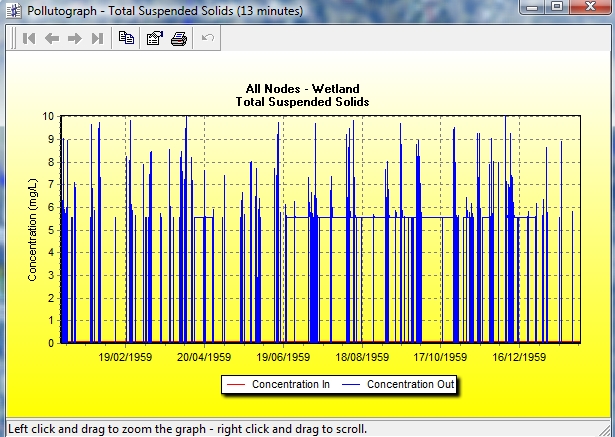
The time series graph below shows inflow and outflow TSS concentrations for a wetland treatment node; the time-step chosen for production of the time series graph is for a 13-minute interval (even though the model was run at a 6 minute time-step). NOTE, however, that the time-step chosen must be equal to or greater than the time-step at which the simulation was run. The concentration spikes correspond to periods of stormflow, the almost constant concentrations correspond to periods of baseflow, and the time-steps with no concentration shown correspond to periods of no flow. When interpreting music output it is important to remember that zero flow › no concentration.
Properties of the graph can be modified using the edit button  . Editable properties include colours, scales and displayed parameters. For example, to change the timeframe shown on the x-axis, click on the Paging panel, and edit the number of points shown per page. To display all data points on the one graph page, set Points per Page to zero.
A graph can be moved, resized (within limits), and captured like any other window. It can also be copied to the clipboard ( ) for pasting into other applications, or sent directly to a printer (
 ).
).
 Tip Box
You can zoom in on a portion of the graph by left-dragging over the required area. You can ‘drag’ the graph along either axis by right-dragging on the graph. You can undo any changes by clicking the ‘Restore to Default’ icon ( ).
).
Water quality standards will be displayed on the graph when they are active. They can be turned on or off using the check boxes on the Water Quality Standards definition box, accessed by the Water Quality Standards command on the Catchment menu.
The Time Series Graph command for Meteorological Data, accessed via the Catchment menu, plots time-step rainfall and daily evapotranspiration data in millimetres against time. No further setup information is required, but the graph format and data shown can be modified using the edit button if required.
Tip Box
When displaying the time series graph of gross pollutants in a gross pollutant trap, the mass of gross pollutants accumulated in the trap is automatically displayed.