Analysis tools
This section describes the Source processing tools and component models that are installed by default in Source. For detailed descriptions of component models, see the Source Scientific Reference Guide.
Mapping Analysis window
The mapping analysis window displays a map of flows and constituent loads per sub-catchment and can be accessed using . The relevant catchment variables need to have been recorded in the Scenario run to be able to view them in the Map Analysis Window. You can perform the following functions in this window:
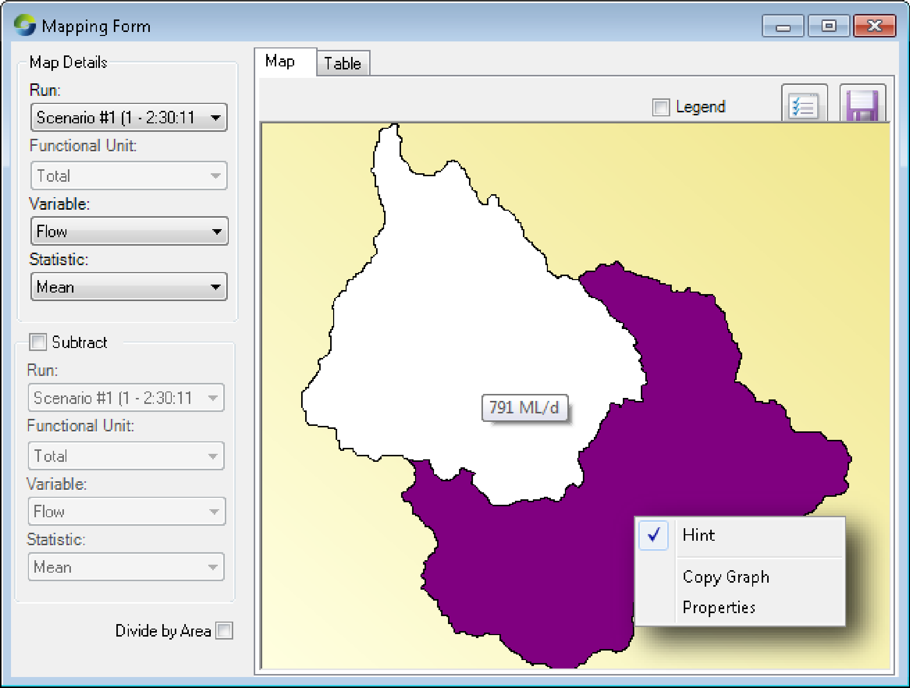
- To display flows and loads in each sub-catchment, under Map Details, click to open the Runs drop-down menu. Choose a scenario, then the desired Variable and Statistic values from the respective drop-down menus. Move the mouse cursor over a sub-catchment in the map view. A tool-tip appears near the mouse cursor, indicating the variable amount for that sub-catchment per year (Figure 1);
- Flows are reported in ML/d and constituent loads in kg/d;
- You can calculate the difference between two scenario runs by enabling the Subtract checkbox. Carry out the same steps outlined above for the mapping analysis window; and
- Display results per unit area by enabling the Divide by Area checkbox. Flow depth is reported in m/s and constituent load in t/km2/y.
Figure 1. Mapping form with tool-tip showing TSS
Data unit converter
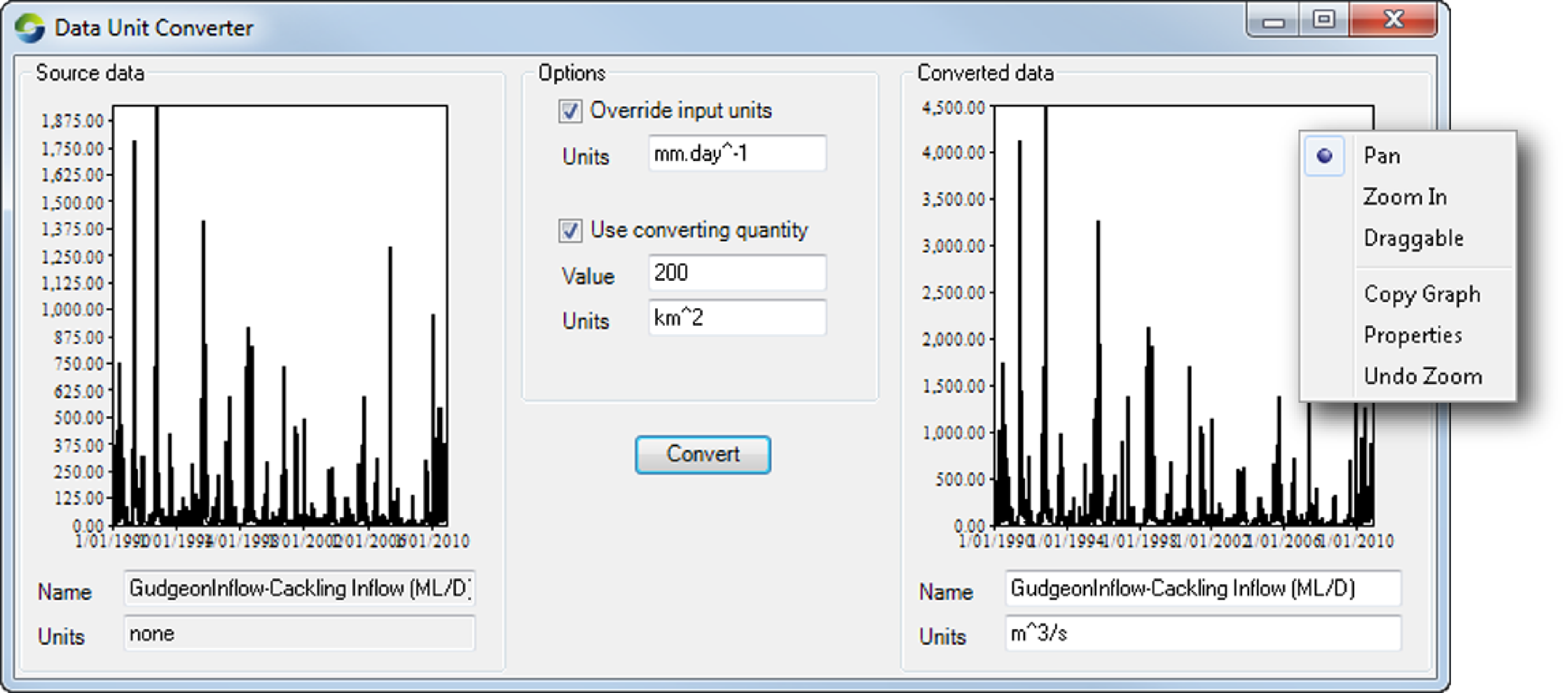
This tool converts units (embedded into data files) in Source from one type to another. You can access it from (Figure 2).
Figure 2. Data Unit Converter
Use the converter as follows:
- Drag and drop a data file onto the Source data window in the left side panel. If there are units in the data file, they will appear in the units field below the input window. If they do not, log an issue into JIRA;
- Enter the output/target units in the Units field on the right side (under Converted Data). You can either use the default name (copied from the source data file) or enter a new name; and
- Click Convert. To save the converted file, you have to drag it somewhere else in Source that has a Save as function. You cannot right-click the converted data graph and save it.
Note that if there are no units in the input file, you must force the data converter to assume that there are input units by ticking the Override input units checkbox and entering the "assumed" unit under Units. For example, you have a CSV file containing dates and rainfall, but it does not contain any units. You want an output containing metres per day. Assume the input is in mm/day:
- Drop the input file into the Source data window;
- Tick the Override units checkbox;
- Enter mm.day-1 into the Units field;
- In the converted data window, enter the name for the converted data set;
- In the converted data window units field, enter m.day-1 (metres per day); and
- Click Convert. The converted data should be scaled down.
You can also scale the converted output to your desired units by ticking the Use converting quantity checkbox. Enter a non-zero value into the Value field and click Convert to scale the output by both the value and the difference in magnitude of the units eg 0.5 mm/h converted to m/h with value 3 ends up being 0.0005 m/h. Note that you must specify both the source value and the target units.
Right clicking in the 'Converted data' window will reveal a pop-up menu of options. This enables zooming, panning, dragging, formatting and copying a picture of the output graph to the paste buffer.
Data calculator
The Data calculator can be used to analyse spatial data and time series through the use of simple arithmetic operators. A single data set or two comparable data sets can be analysed using the data calculator. In Source, you can access it using .
You can use rasters, time series or numbers as operands:
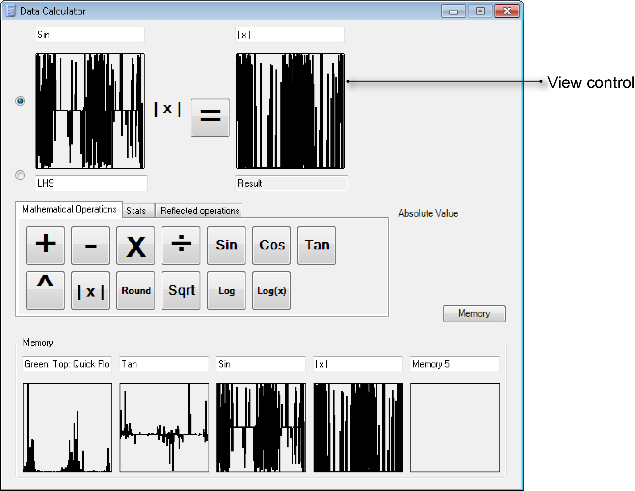
- Drag and drop raster data or time series into either of the two view controls (raster or time series are displayed in a small window called a View Control (Figure 3) or use a combination of a raster/time series and a number.
- Use the radio buttons to select either the view control or numeric values as left and right operands.
- Click one of the basic operations buttons (addition, subtraction, square root etc). The data calculator displays the operand you selected.
- Click =, and the result, either raster/time series or numeric, appears in the results area on the right.
The memory feature of the data calculator allows you to save previous results, either numeric or raster/time-series.
Click Memory to open the memory area. To save a result raster/time series into the memory, click on the 1st or 2nd operand, or result, view control, then drag and drop the contents into your desired memory view control. The label above each view control resides shows the mathematical operation leading to the result stored there. Figure 3 shows the memory area with several stored results.
Figure 3. Data Calculator with data stored in memory
To save any of the results, right-click any of the view controls, and choose Save from the pop-up menu. You can also drag the contents of any view control into any other view control or graph form anywhere else in Source.
The Stats tab gives a statistical summary of the data sets that have been analysed with the Data Calculator. The Reflected Operations tab provides additional data manipulation operations, such as Merge, find Maximum value or multiply two rasters. It allows you to perform customised operations. You can use a plugin to create these operations, which then appear on the list, and can be performed on various data sets.
Data modification tool
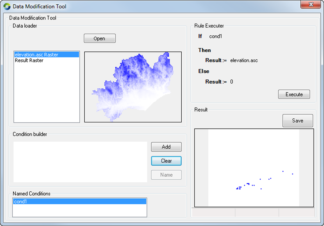
The Data modification tool allows you to edit data inputs depending on conditions that you wish to specify. Choose Tools » Data Modification Tool to open the tool, as shown in Figure 4 and carry out the following steps to change the data inputs:
- Click Open under Data loader, which displays the file name in the box below, along with the file on the right;
- Under Condition builder, click Add to add a condition. Modifying the input data, conditional operator and condition value can be accessed by hovering and clicking on the relevant area in the condition builder. A drop-down menu appears.
- Click Name to associate a name with the condition;
- Clear can be used to clear the list of conditions if it gets too long and is no longer required.
- Under Rule Executer, you can specify the output for specific aspects of the input. For example, if the condition reaches a certain value, the result will be 0.
- Click Execute, ad the output will be displayed in Result, which can be saved by clicking Save.
Figure 4. Data modification tool
Graph Control
Choose Tools » Graph Control to open a charting tool window, which can be used to drag data and display it. Refer to Using the Charting Tool for details.
Regression tests
Regression tests ensure the following:
- Changes (such as bug fixes) on Source do not introduce additional problems;
- Old projects are compatible with future versions of Source; and
- Correct results are not inadvertently changed due to software changes.
A detailed description on working with regression tests can be found at /wiki/spaces/SD41/pages/25822617.
There are three sub-menus under Tools » Regression tests that allow you to create and run regressions tests locally. The first step is to set up the regression test project and build the test using the Scenario test builder.
1 Scenario Test builder
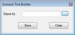
The Scenario test builder (Figure 5) allows you to create a folder that will contain all the regression test files for a project:
- Prior to running a scenario, ensure that you have recorded the parameters relevant to your test;
- Once you have run a scenario, ensure that all the recorded results show the correct results. Open the Scenario Test Builder (using Tools » Regression Tests » Scenario Test Builder); and
- Click on the ellipsis button and load the folder containing the results of the regression tests. Click Save to save the folder location or Clear to load a different folder. This test folder contains sub-folders for each scenario within your project containing the expected results or baseline files. This folder also contains a Source project file that the regression test loads and runs to compare to the baseline files.
Figure 5. Regression tests, Scenario Test builder
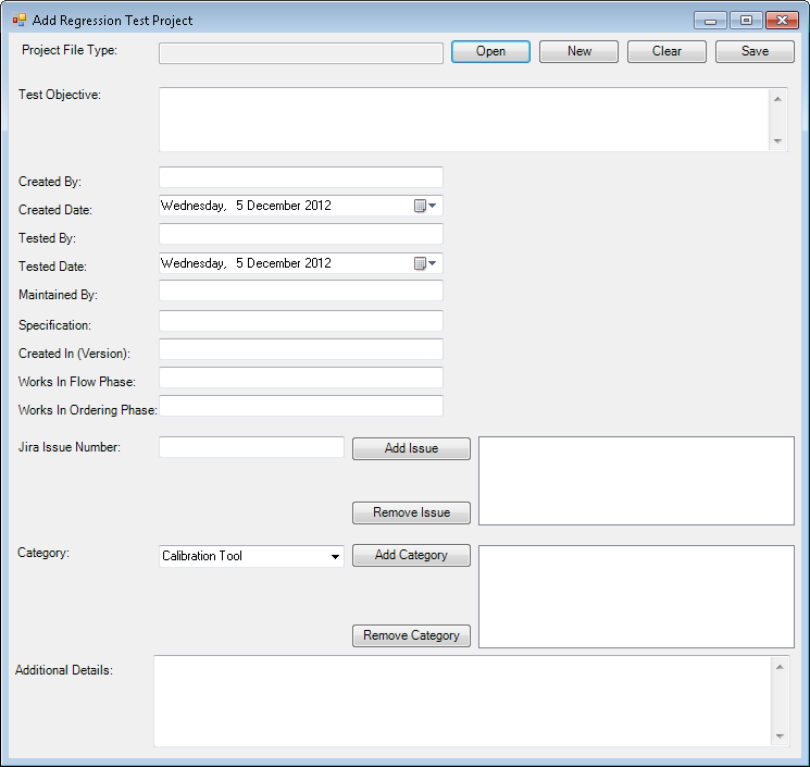
2 Create/Edit Regression Test Description file (.xml)
This allows you to document information about the test files that were saved in the scenario test builder. It tells you what functionality each file is testing and is saved in XML format.
Choose Tools » Regression Tests » Create/Edit Regression Test Description file (/xml) to open the Add Regression Test Project dialog (Figure 6). Once you have entered as much information as you can, click Save.
Figure 6. Regression tests, Add regression test project
3 Test Runner
The test runner allows you to run various tests on scenarios:
- Choose Tools » Regression tests » Test Runner to open the dialog shown in Figure 7;
- Click on the ellipsis button to load a folder containing the errors; and
- Click Run to run the scenario.
Click the Show less Info. button to view fewer details on the errors. The Export All Errors button allows you to save the errors to a file.
Figure 7. Regression tests, Test Runner
