Constituents
Constituents refer to materials that are generated, transported and transformed within a catchment and affect water quality. Common examples include sediments, nutrients and contaminants, such as salt or dissolved solids. Processes that act on these constituents to generated, transport and transform them can be modelled in Source. These models are categorised into:
- Constituent generation models - describe how constituents are generated in the functional unit and the resulting concentrations or loads delivered to the sub-catchment node;
- Constituent routing (conservative constituents) models - describes the movement of constituents along a river channel network, including exchange of constituent fluxes between floodplains, wetlands, irrigation areas and groundwater;
- Constituent filtering models - represent any transformation of constituents between generation within the FU and arrival at the link upstream of the sub-catchment node.
This chapter begins with an explanation of how to configure constituents at nodes and links in Source, and then discusses each of the models listed.
Defining constituents
Constituents can be defined in step 4 of the Geographic Wizard, or by choosing (Figure 1).
Figure 1. Configure constituents
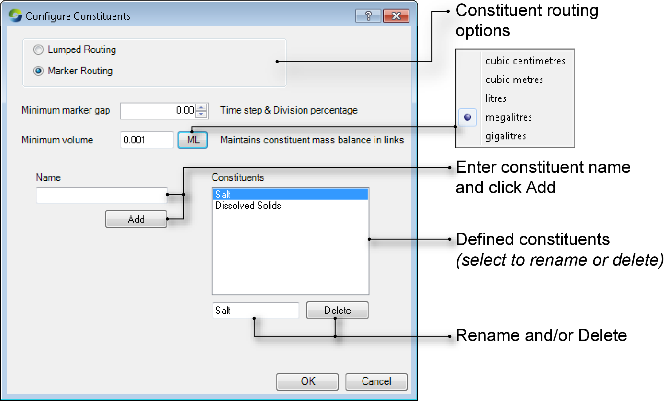
Refer to Constituent routing for choosing the type of constituent routing desired. The following parameters must also be configured in this step:
- Minimum Marker Gap - defines the spacing between markers as either a fraction of the model time-step or fraction of the reach division. This parameter can improve model efficiency by reducing the number of markers that require processing at each model time-step. The allowable range is from 0 to 1, with 0 not deleting any markers, while a value of 1 will ensure that at the end of each time-step, there is only one marker defined for each reach division; and
- Minimum volume to maintain constituent mass balance within the links.
Once you have defined constituents, they can be configured for individual nodes. This is described next.
Configuring constituents at nodes
In Source, the behaviour of constituents at each node varies. Select Constituents in the node’s feature editor to configure them. Depending on your requirements and the type of node, you can specify either a constituent’s load or concentration at a node. For example, you can only specify a constituent’s concentration on an inflow node.
Inflow node
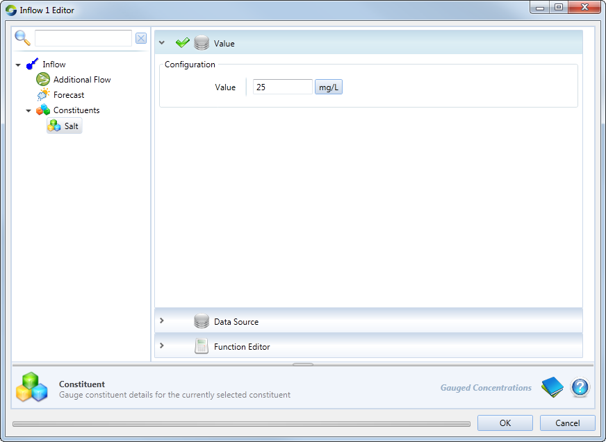
Figure 2 shows the item in the feature editor, where you specify the inflow constituent data (as a concentration), which can be entered as a single value, as a time-series file (using Data Sources) or through the Function Editor. This behaviour is similar to flow.
Figure 2. Inflow node (Constituents)
Gauge node
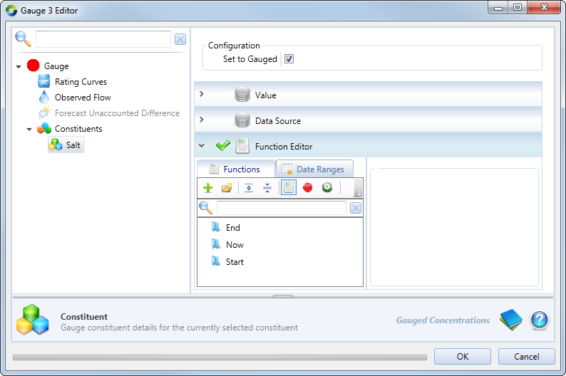
If using gauge flow to override modelled flow, then leave as modelled, and constituent loads will be calculated using the gauged data concentration. Enabling the Set to Gauged checkbox allows you to set up the modelling of constituents as a single value, a data source, or as a function. Disabling the checkbox will allow the constituents to flow through the node.
Figure 3. Gauge node (Constituents)
Storage node
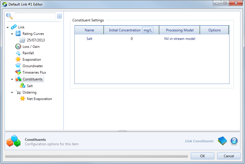
You must also define the initial concentration of each modelled constituent in the node’s feature editor, under Constituents (Figure 4). You can also specify the following constituents (using the contextual menu) on a storage routing link:
- Additional Inflow load - additional constituents that flow in;
- Gauged Concentrations - override the the modelled concentration and replace it with gauged concentration; and
- Groundwater - additional constituent (flow with a concentration) that comes into the storage.
Figure 4. Storage node (Constituents)
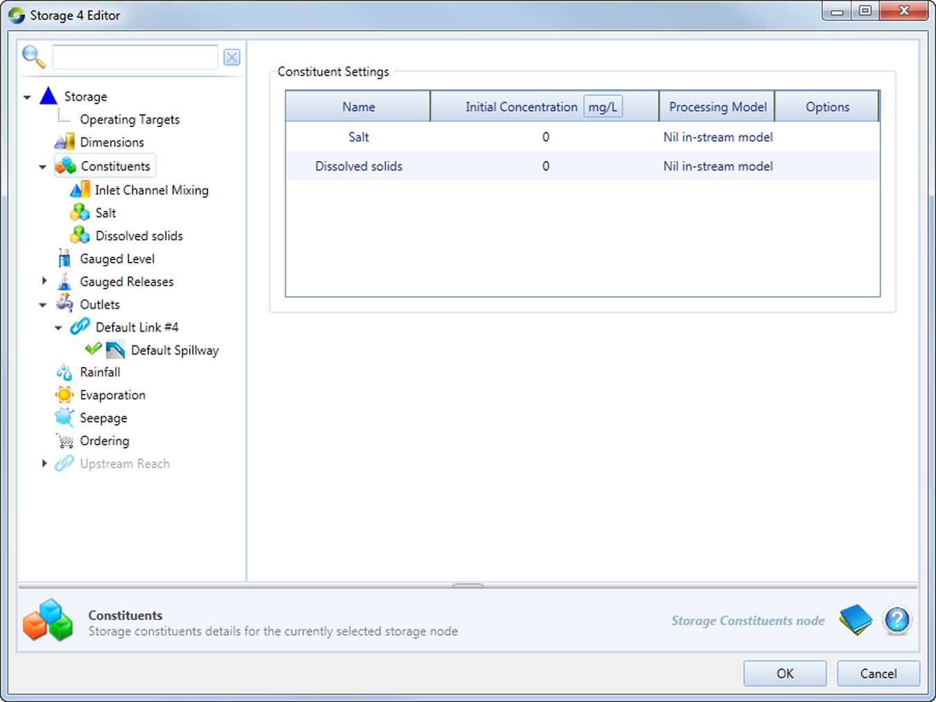
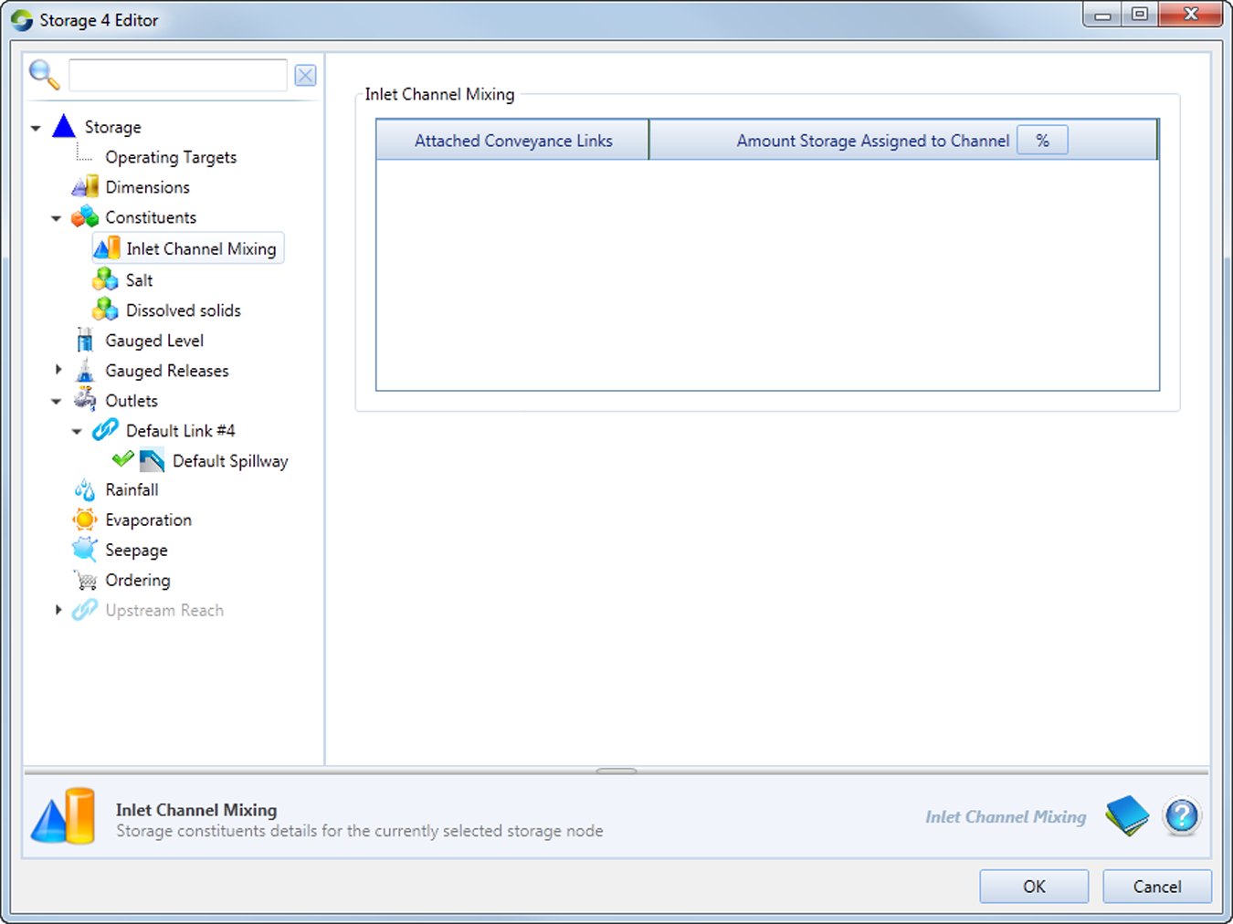
Inlet channel mixing allows you to introduce mixing of constituents at a conveyance link (Figure 5). You specify a percentage of the wetland/storage volume that is conceptually represented by the conveyance link, and the remaining volume represents the main body of the storage/wetland. When exchange of water occurs between the wetland/river or the wetland/wetland, mixing of constituents is assumed to occur in the inlet channel. If the exchange of water is large enough to flush out the inlet channel, then the constituents will mix with the main body of the wetland, or the river depending on the direction of water exchange.
Figure 5. Storage node (Inlet channel mixing)
Links
Initial Concentration (Figure 6) refers to the link’s constituent concentration when the simulation begins. This parameter assigns a concentration for each modelled constituent in the scenario for the markers created in that link during the model initialisation. Right click on Constituents, and you can also load a time series to specify the following (using the contextual menu) for a storage node:
- Additional Inflow Load - this is specified as a load, and is similar to the parameter in Links;
- Groundwater - specified as a concentration, same as for Links; and
- Timeseries Flux - this is also configured as a concentration.
Figure 6. Storage Link Routing (Constituents)
Configuring CG models
Constituent generation models describe how constituents (eg sediments or nutrients) are generated within a functional unit and the resulting concentrations or loads delivered to the sub-catchment node. In Source, they can be configured using the Geographic Wizard or by choosing the Edit menu commands. To configure the models in Source, first define the constituents and then parameterise them. This is described next.
Assign constituent models
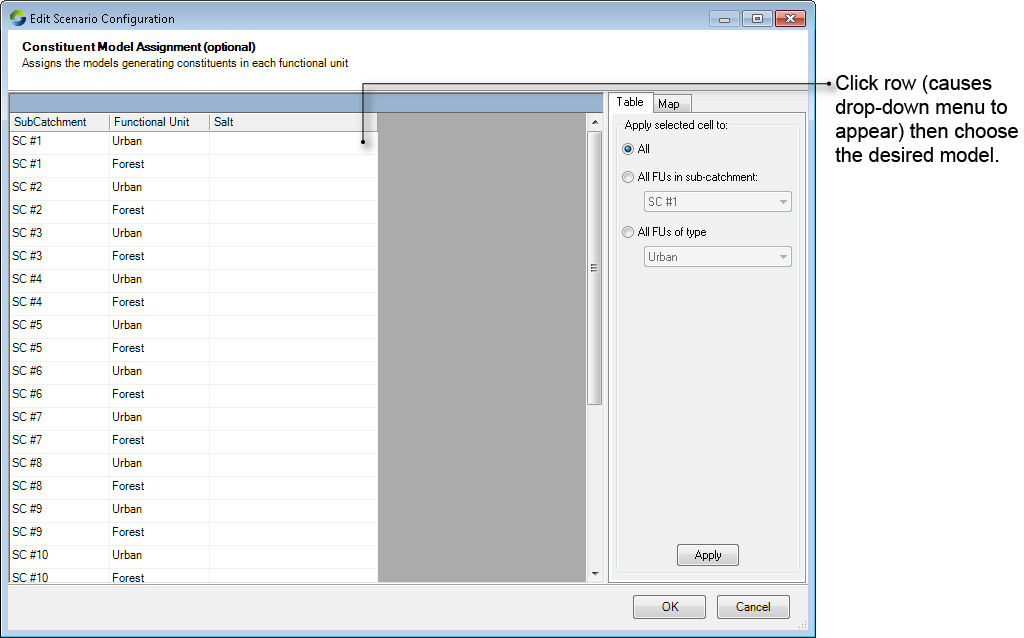
You can assign constituent models by choosing . The number of columns in the resulting window (Figure 7) will depend on the constituents you defined. Choose the desired model from the drop-down list in each constituent column.
Figure 7. Assigning constituent models
Parameterise CG models
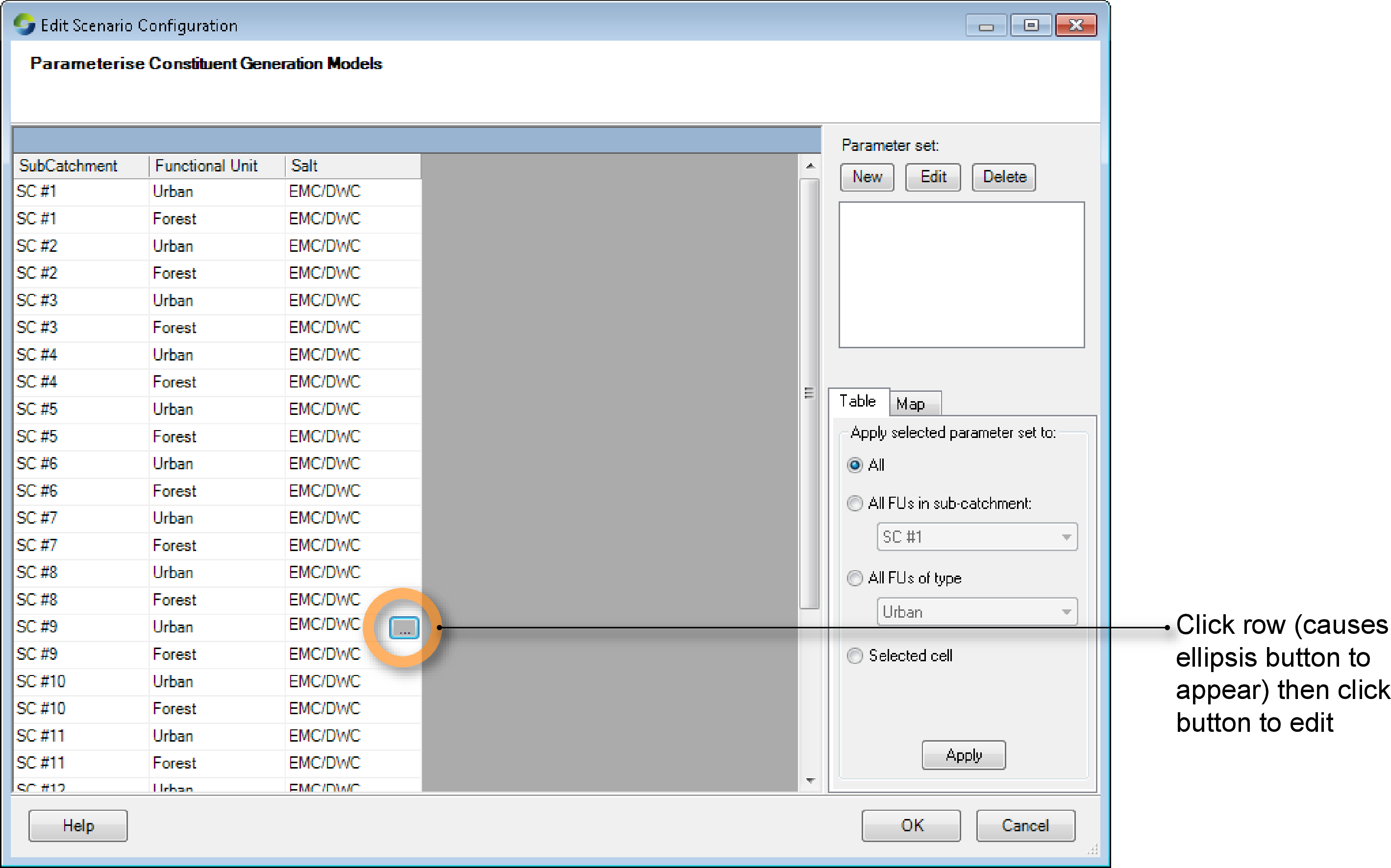
You can parameterise constituent generation models by choosing (Figure 8). This can be done using parameter sets and is similar to that for rainfall runoff parameterisation. You can also use a Hazard Map, which requires the Spatial Data pre-processor plugin. This plugin is available through the Plugin Manager in the Tools menu. See Spatial data pre-processor for information on the plugin and Hazard Map Scaling.
Hazard maps are useful for informing catchment and land managers of parts of the landscape that are most vulnerable to certain environmental hazards, such as soil erosion or salinity. Scaling EMC and DWC values using a Hazard Map allows areas with "hazardous" land uses (eg highly grazed areas can be susceptible to higher levels of soil loss) to reflect the expected constituent magnitudes in such areas.
Figure 8. Parameterise constituent generation models
Constituent routing
In Source, routing of conservative constituents can be undertaken using a marker tracking method (Close, 1996). Markers, representing constituents, are created at defined locations in the schematic and their downstream movement is modelled to determine concentration at model components. These concentrations are adjusted for rainfall, evaporation and inflows from tributaries and groundwater systems. Refer to the Source Scientific Reference Guide for more information.
There are two types of constituent routing available as shown in Figure 1:
- Lumped routing is the simplest approach, where conservative constituents are routed within a link based on kinematic wave theory. Assuming fully-mixed conditions within a link, the constituent flux and concentration simply moves from the top of a link to the downstream end of a link within a time-step, preserving the mass balance. Constituent concentrations in a link can be altered by the addition of constituents generated from sub-catchments, external inflows, and losses within a reach; and
- Marker routing considers conservative constituents as particles and tracks their movement within a link, which can be divided into divisions for hydrologic routing purposes. Initially, the model will start with a marker at the end of each division in every link. At every time-step, a new marker for each constituent will be created for each division, and the distance a marker moves is driven by the velocity in the division over the current time-step. While the flow rate is assumed constant over the time-step, the velocity within the division will change as a result of change in reach storage and cross sectional area. Markers will travel through the river network until they are either merged with adjoining markers, or leave the river network (ie via extractions, decay within the reach, evaporation, groundwater inflows/losses and rainfall).
Configuring filter models
Filter models represent any transformation of constituents between generation within the FU and arrival at the link upstream of the sub-catchment node. Filter models process constituents within the FU and as with constituent generation models, are applied to FUs. Note that only one filter model can be applied to a sub-catchment/FU combination. The configuration of two filter models in particular have been described - Farm dams and the RPM pre-processor.
Just as with CG models, filter models can be assigned and parameterised (optional) using the Geographic Wizard or the Edit menu commands.
Assign filter models
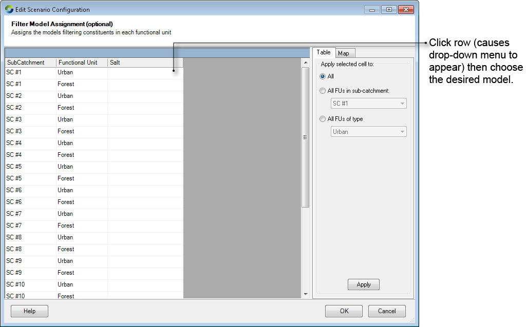
Choose to assign filtering models to a scenario. Figure 9 shows the resulting window.
Figure 9. Assigning filter models
Parameterise filter models
There are two ways of assigning parameters sets to each filter model for any combination of sub-catchment, FU and constituent.
You should use the FU TEDI Preprocessor only when you specifically model the impact of farm dams within your catchment. For configuration details on the Farm Dams pre-processor, see Farm Dams. Use the next method when you have any other filter models applied.
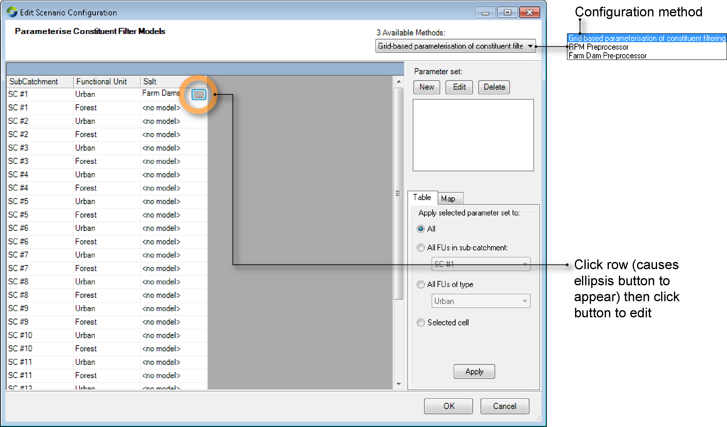
The method for parameterising filter models using grid-based parameterisation is similar to that for rainfall runoff and constituent generation models. Figure 10 shows the window to parameterise filter models.
Figure 10. Parameterise filter models
Farm Dams
This model works by capturing or filtering a proportion of runoff within each FU according to the total storage density of dams.
Overflow from dams in one FU will contribute to the total runoff of all FUs within a sub-catchment. The Farm Dam model is able to estimate the impact of farm dams on stream flow at catchment scales (up to several hundreds of square kilometres in area). There are several input data requirements that are required to set up a farm dam model. Refer to the Source Scientific Reference Guide fore more information.
Filter models act on constituents, so when you develop a scenario, you need to add a constituent that represents any runoff that is potentially captured (or could be captured) by farm dams (eg. called Flow). The Farm Dams model will then be applied to this constituent. Alternatively, if you do not add a specific Farm Dams model constituent, you can still apply the Farm Dams model to any other constituent, regardless of name.
 It is recommended that you do NOT model constituents in conjunction with modelling farm dams, as the Farm Dams model may adversely impact constituent loads and concentration calculations. If you wish to apply th model to an existing scenario, make a copy of the scenario before running the Farm Dams model, so that existing scenario water quality simulations are not affected by the altered runoff. |
When modelling farm dams, you should initially use the Geographic wizard to create a scenario without the Farm Dams model. This scenario is then your base case. You can then make a copy of the scenario, rename it, and apply the Farm Dams model to the copy of the original scenario and parameterise from the Edit menu. By having a separate base case and "farm dam" scenario, will allow the impact of farm dams on surface water runoff to be quantified. |
To assign a farm dam model to a FU, choose . In the constituent column, choose Farm Dam from the drop down menu. You can also decide which sub-catchments and FUs to assign this model to using the Map tab.
To parameterise the Farm Dams model:
- Choose
- From the Available Methods drop-down menu, choose Farm Dam Pre-processor (Figure 11);
- Select the flow constituent or other constituent that the farm dam model will be applied to; and
- Select the functional unit that the farm dam model will be applied to. Each functional unit can have different farm dam parameters, such as different size class/volume relationships, demand factors, densities etc;
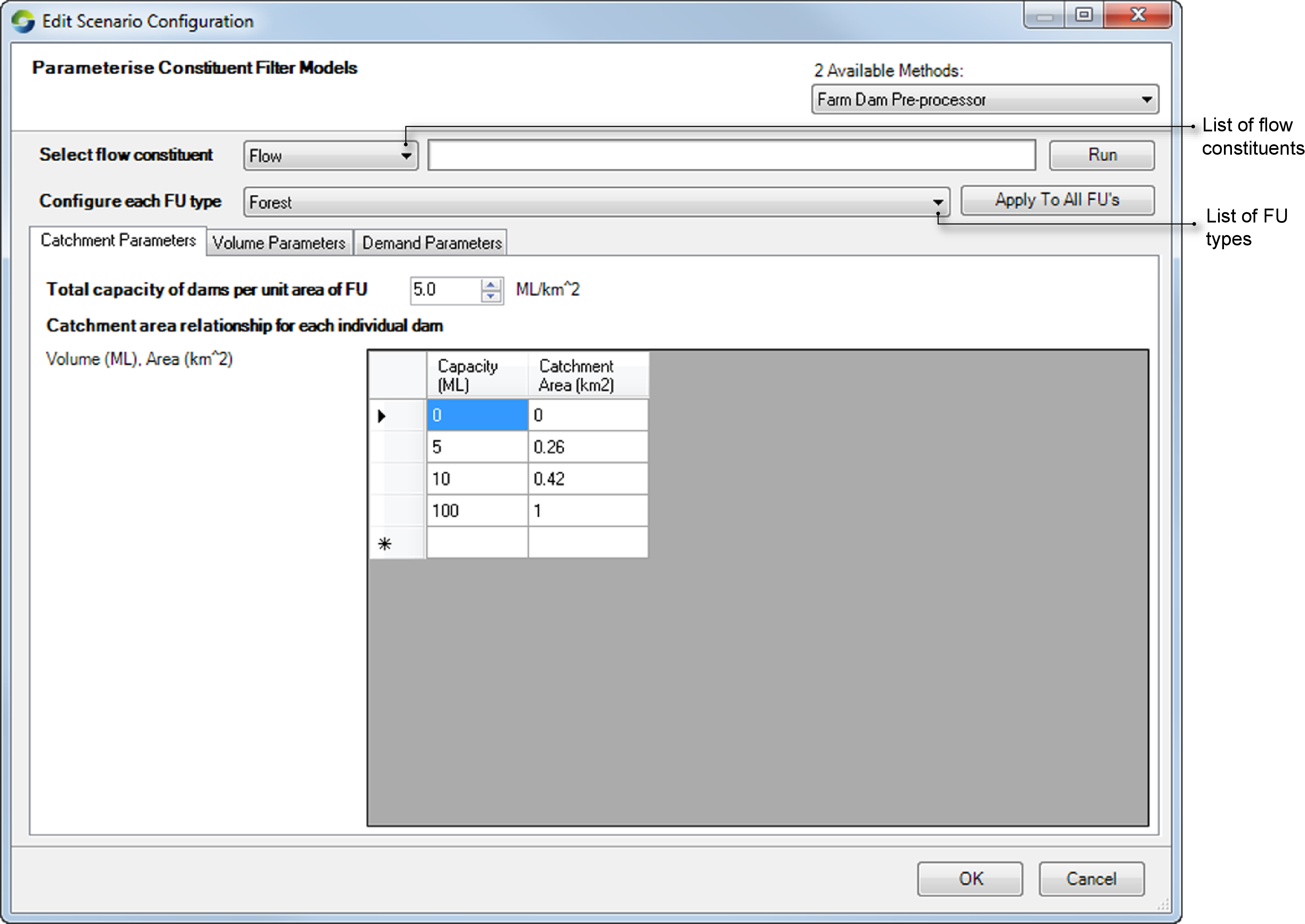
Figure 11. Farm dam pre-processor, Catchment parameters
Next, use each of the three tabs to configure various properties of the dam.
Click the Catchment Parameters tab to specify the catchment related properties of the dam:
- Set the total capacity of dams per unit area of FU, ie the number of megalitres per square kilometer.
- In the dam capacity-catchment area relationship table, specify the catchment area/volume relationship for each individual dam: for each dam, add one row to the table. This function represents the upstream catchment area corresponding to a 5, 10 and 100 ML dam (default). You can specify additional capacity groupings if necessary.
- To delete rows from the table, click the grey cell at the start of the row, then press Delete; and
- To add rows to the table, click the grey cell containing the
 at the bottom of the table.
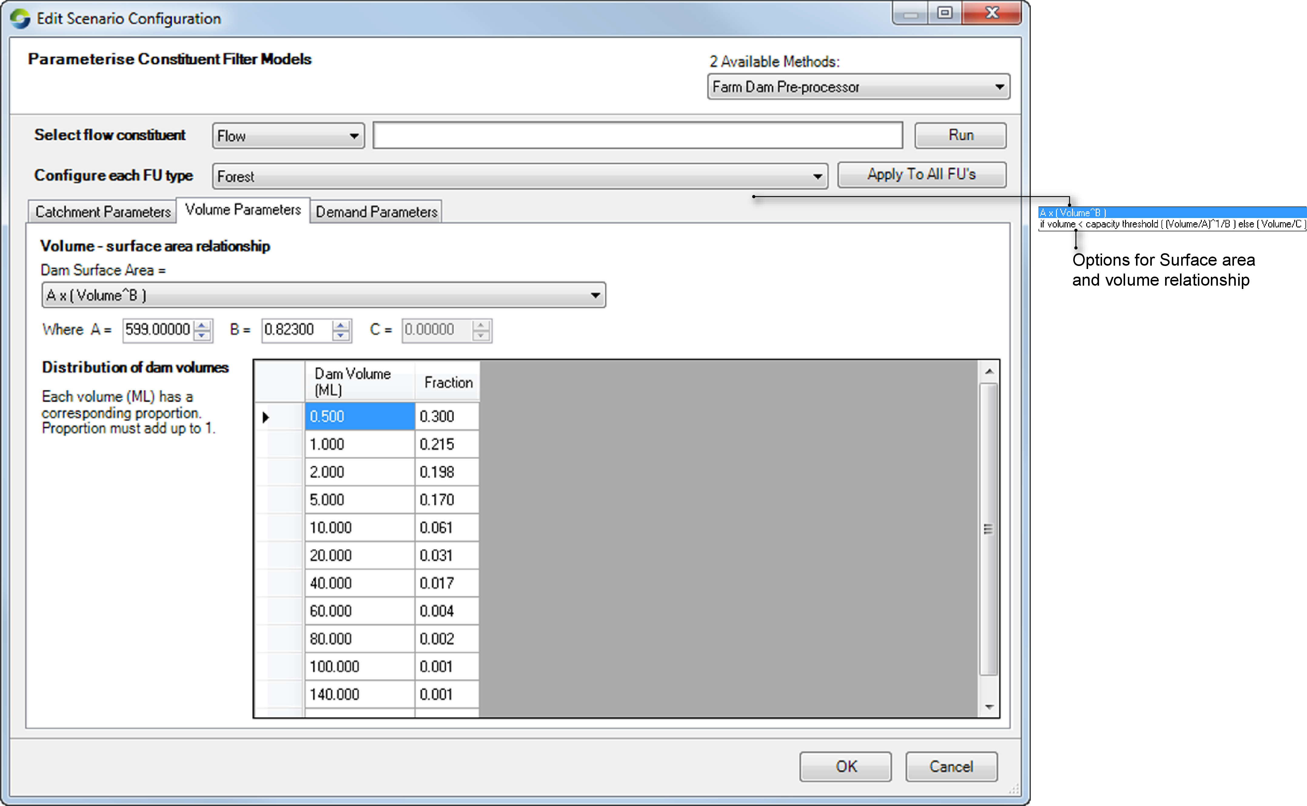
Use the Volume parameters tab to:
- Select the type of function to define the surface area/volume relationship;
- Specify the values for the surface area/volume relationship parameters A and B (Figure 12);
- Specify the farm dam size class/volume distribution function. This function will be used by the pre-processor to stochastically generate a sample of farm dams based on the density and size class distribution given in previous steps;
- The Dam Volume column can be changed to have any number of values by deleting or adding cells. To delete a cell, overwrite the current value with zero and press Enter; and
- The Fraction column of the size class/volume distribution must sum to 1.
Figure 12. Farm dams, Volume parameters
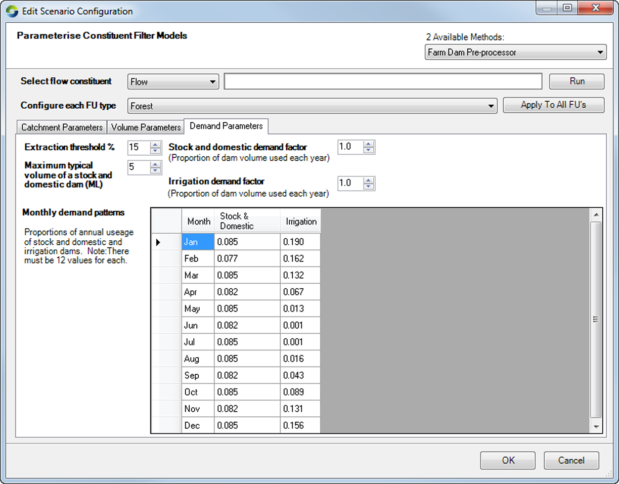
Click on the Demand Parameters tab. Several constant values can be specified in Figure 13:
- Extraction threshold - this is the threshold below which no more water can be extracted from a farm dam (effectively the dead storage of a farm dam). The default value is 15%, which specifies that when the farm dam is at 15% of its total capacity, no more water can be extracted from the dam;
- Maximum typical volume of a stock & domestic dam. The capacity threshold between large irrigation dams and smaller stock & domestic dams (The default is 5 ML);
- Demand factors - the proportion of water used as a proportion of dam volume. Some dams may be used frequently, and the water constantly replenished, whereas other dams may not be used at all. This proportion is the average usage factor for all catchment dams (The default is 1); and
- Monthly Demand patterns - extraction from farm dams are typically seasonal, thus water usage rates are modelled with a set of average monthly demand values. The monthly values must sum to 1.
Figure 13. Farm dams, Demand parameters
To remove the Farm Dams model for all FUs of a particular type, set the total capacity of farm dams per unit area of FU to zero, then click Run. The Farm Dam models will be removed from the currently selected FU type.
Once all the values for the Farm Dam models for each FU have been entered, click Run to start the pre-processor.
If you change a parameter, and re-run the pre-processor, the previous model parameters are overwritten. If you wish to experiment with different parameters, make a copy of the base scenario, rename the copy, then change the parameters in the copied scenario.
RPM Filter
The Riparian Particulate Model (RPM) quantifies the particulate trapping in riparian buffers through simulation of the processes of settling, infiltration and adhesion. It consists of three components that simulate particulate trapping:
- Coarse particulates by settling;
- Fine particulates by adhesion; and
- Fine particulates by infiltration.
To use RPM in Source, you must first define the catchment network using a DEM and allocate FUs using a land use map.