Groundwater interaction module
Introduction
The Groundwater Interaction module in Source is a collection of modules and protocols/guidelines that simulate the exchange of groundwater and salt between rivers and the underlying groundwater systems.It determines the exchange flux of water between a river and the underlying aquifer for each link of Source at each time-step. The estimated flux accounts for interactions between groundwater and surface water along the entire length of the link. The direction of the flux can either be from the river to aquifer or vice versa, that is, the river either loses water to the groundwater system or it gains water from the groundwater system.
The various components of the exchange flux may be calculated within Source or they can be imported as a time series from field monitoring. The exchange fluxes may include the following components:
- Continuous natural exchange between the river and the aquifer, which is driven by the head difference;
- Flux out due to evapotranspiration;
- Flux out due to groundwater pumping;
- Flux in due to irrigation and diffuse recharge; and/or
- Exchange fluxes during (within bank and overbank) flood events.
The exchange fluxes are assigned to a Source link, once:
- Storage routing has been enabled on the link (refer to Types of link routing); and
- Groundwater has been enabled in the scenario using Edit » Enable Groundwater.
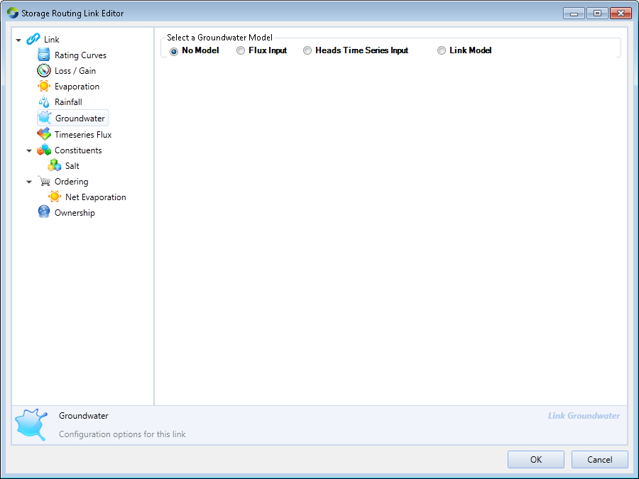
Open the link’s feature editor and choose Groundwater from the list. Figure 1 shows a scenario where no groundwater model has been selected. This is the default option, and shows that Groundwater-Surfacewater modelling is not yet enabled.
Figure 1. Link (Groundwater, no model)
Types of groundwater models
There are three types of groundwater models which can be configured in Source, which are described next. A positive flux represents a discharge out of the river while a negative flux represents a recharge into the river.
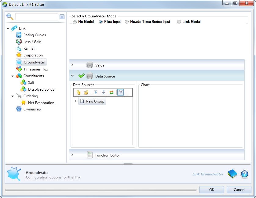
Flux input model
This represents the daily exchange flux between the reach and its aquifer, which can be specified as a single value, by uploading a time series (using Data Sources), or via an expression using the Function Editor (Figure 2). Note that flux values can be both positive and negative, so the reach alternates between gaining and losing.
Figure 2. Link (Groundwater, Flux Input)
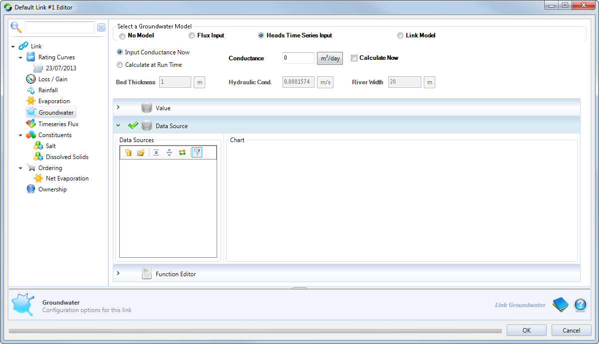
Heads Time Series input
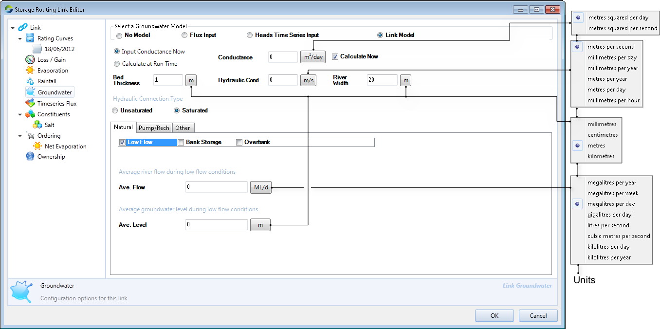
One method for estimating the groundwater flux is based on knowledge of the head difference between the river stage and the water table in the underlying aquifer. The Heads Time Series input model (Figure 3) uses the head difference between the current calculated river stage height and the interpolated (from rating curve) groundwater head to calculate groundwater flux. It requires:
- A rating curve to determine river stage height from river discharge (refer to Link rating curve);
- A time series of groundwater heads covering the period of simulation (which can be specified as a single value, via a file using Data Sources, or via an expression using the Function Editor); and
- A conductance value (either set or calculated prior to run time, or calculated dynamically at run time). Enabling the Calculate Now checkbox allows you to specify three additional parameters (Bed Thickness, Hydraulic Conductance, and River Width) which are used to calculate conductance.
Figure 3. Link (Groundwater, Heads Time Series Input)
Link model
There are two types of hydraulic connections available when choosing this type of groundwater model - unsaturated and saturated. The former is used when there is a permanent unsaturated connection between stream and the adjacent aquifer, that is, the stream must always be a losing one. The latter is the most complex of all the groundwater models. Both are described next.
The Unsaturated Connection model (Figure 4) uses the head difference between the stream and the aquifer, together with a conductance value to calculate the groundwater flux. There are three main steps to configuring the model:
- Load a rating curve and set stream (link) height;
- Enter a conductance value (similar to Heads Time Series Input) ; and
- Set the groundwater level as a long term average groundwater level, or via a simple forecast model. Note that groundwater level must always be either be either greater than or less than the river level, thus being a gaining or losing reach.
A groundwater head value that is larger than the current stream height generates a flux from the aquifer to the stream (a negative flux) and a groundwater head value that is lower than the stream height generates a flux from the stream to the aquifer (a positive flux).
In a Saturated Connection model, you may select any of the eight distinct groundwater and floodplain processes to run simultaneously. At each time-step the model evaluates the impacts of each selected process and uses assumed linearity and superposition to aggregate the impacts and calculate a flux.
The parameters for the saturated connection model fall into one of two categories:
- Shared parameters include rating curves, conductance, aquifer transmissivity and aquifer storage coefficient. These parameters are only set once per link and are shared by all of the individual processes in the model. Note that salt concentration can be specified in Constituents (FIGURE).; and
- Unshared parameters only pertain to a single process. For example, average river flow during low flow conditions and average groundwater level during low flow conditions are unshared parameters as they are only relevant for the Low Flow process.
To add a process to the current saturated connection model, enable the desired checkbox. Conversely, to remove a process, disable the corresponding checkbox. The eight processes are described next.
Low Flow
Refer to Figure 4.
Figure 4. Link (Groundwater, saturated, low flow)
Bank Storage
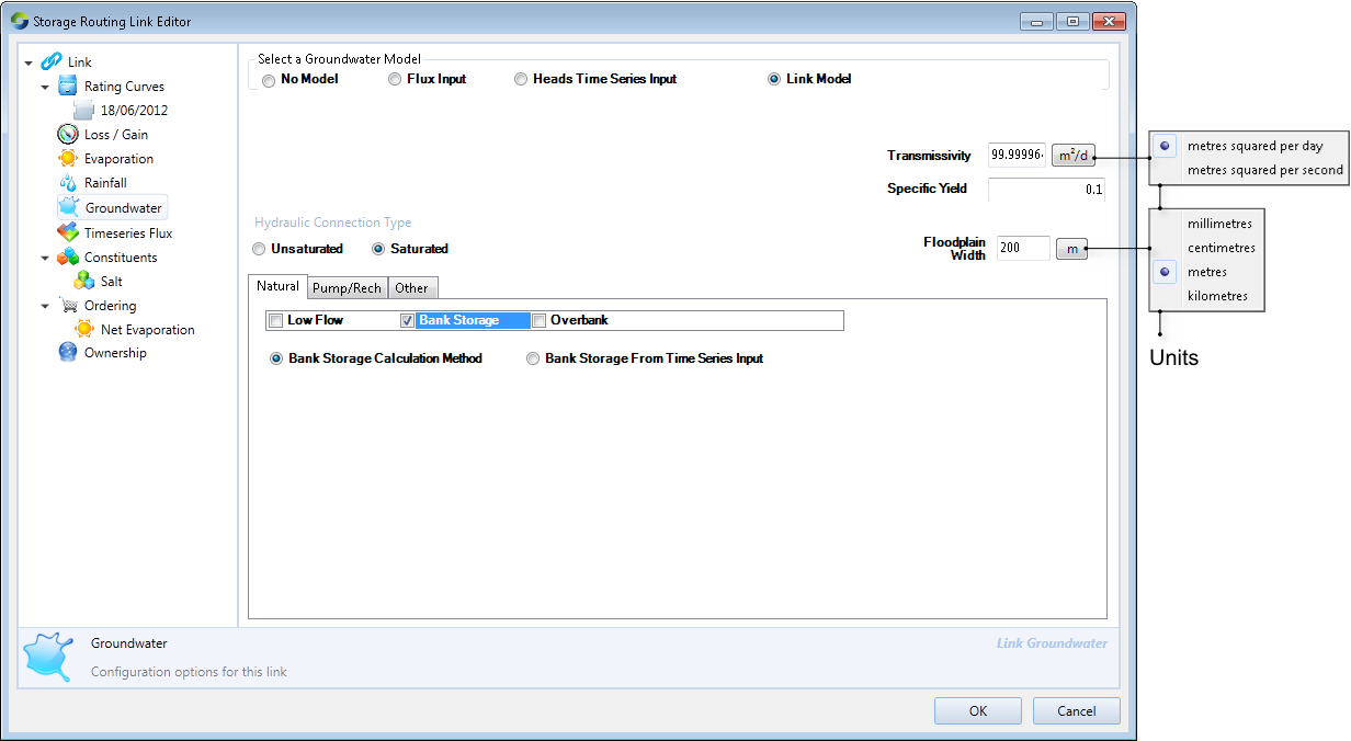
There are two ways to generate a bank storage flux. The first method (Calculation Method - Figure 5) calculates the bank storage flux at run time from shared aquifer parameters and stream flow. At each time-step, the model takes the current stage height for the stream, the previous stage height for the stream, the floodplain width, aquifer transmissivity and aquifer diffusivity, and calculates a bank storage flux.
Figure 5. Link (Groundwater, saturated, bank storage, calculation)
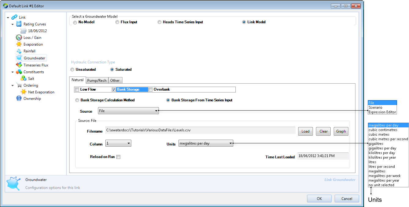
The second method (Figure 6) involves loading a known time series of bank storage fluxes, similar to that done with fluxes and heads. At each time-step, the model will then retrieve a bank storage flux value and add it to the total groundwater flux generated by the other saturated connection model processes.
Figure 6. Link (Groundwater, saturated, bank storage, time series)
Overbank
Overbank (Figure 7) occurs when the stream stage height exceeds the height of the stream bank. Water flows over the stream bank and out onto the adjacent floodplain filling up any depressions and channels and creating inundated floodplain areas. The water in the inundated floodplains either evaporates or infiltrates through the soil and finds its way back to the stream. At each time-step the model determines:
- Whether an overbank event has occurred;
- How much water is in any of the inundated floodplain areas;
- How much of this water is lost to evaporation; and
- How much water is returned to the stream (as a groundwater flux).
Figure 7. Link (Groundwater, saturated, overbank)
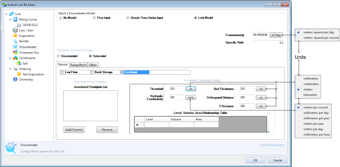
For each inundated floodplain area that you wish to model, an additional six parameters are required:
- Threshold - a (unique) height (in mAHD) that river stage height must exceed to increase the area’s water volume;
- Hydraulic conductivity - the hydraulic conductivity of the surface soil in the area;
- Bed thickness - the bed thickness (surface soil depth in meters) of the area;
- Orthogonal distance - the orthogonal distance (m) from the area centroid to the stream;
- Y distance - the distance from the area centroid to a line perpendicular to the stream through the upstream node (not currently used by the model but included for completeness); and
- A table of level, volume, area relationships for the area such that, in each successive row of the table, the level is greater than that in the previous row and all level values are greater than the threshold.
Pumping
Groundwater pumping is one of the most important processes that impacts the exchange flux between groundwater and surface water. Pumping-induced river depletion is defined as the reduction of river flow due to induced infiltration of stream water into the aquifer or the capture of aquifer discharge to the river. During pumping, while the cone of depression progresses towards a nearby river, groundwater depletion occurs. When this cone reaches the river, the rate of groundwater discharge to the stream reduces, and surface water may even start to infiltrate into the aquifer thus marking the start of river depletion.
After a long period of pumping, the cone of depression takes its final shape (ie a steady-state is reached), and a portion, or in some cases, all of the pumping will be balanced by a reduction in, or reversal of flow, from the aquifer to the river. The proportion of pumping met by river depletion in the steady-state case will depend on various factors, including the proximity of the bore to the river compared to the distance between the bore and other stresses to the groundwater system (eg recharge, ET).
Source allows for two types of groundwater pumping:
- Pumping from an unconfined aquifer (Figure 8) with or without a no-flow boundary - This caters for pumps which tap directly into an aquifer (with or without a no-flow boundary) which is hydraulically connected to the stream. The pump is at a given distance from the stream, it switches on at some time, pumps at a constant rate for a period (the pumping period may occur prior to the simulation start time and the effects are still modelled) and then switches off; and
- Pumping from a semi-confined aquifer (Figure 9) - used to model pumps which tap into a semi-confined aquifer which is hydraulically connected to the stream. Again, the pump switches on at some time, pumps at a constant rate and switches off.
You could enter the parameters for each process, or import a .csv file containing this information.
Figure 8. Link (Groundwater, saturated, unconfined pumping)
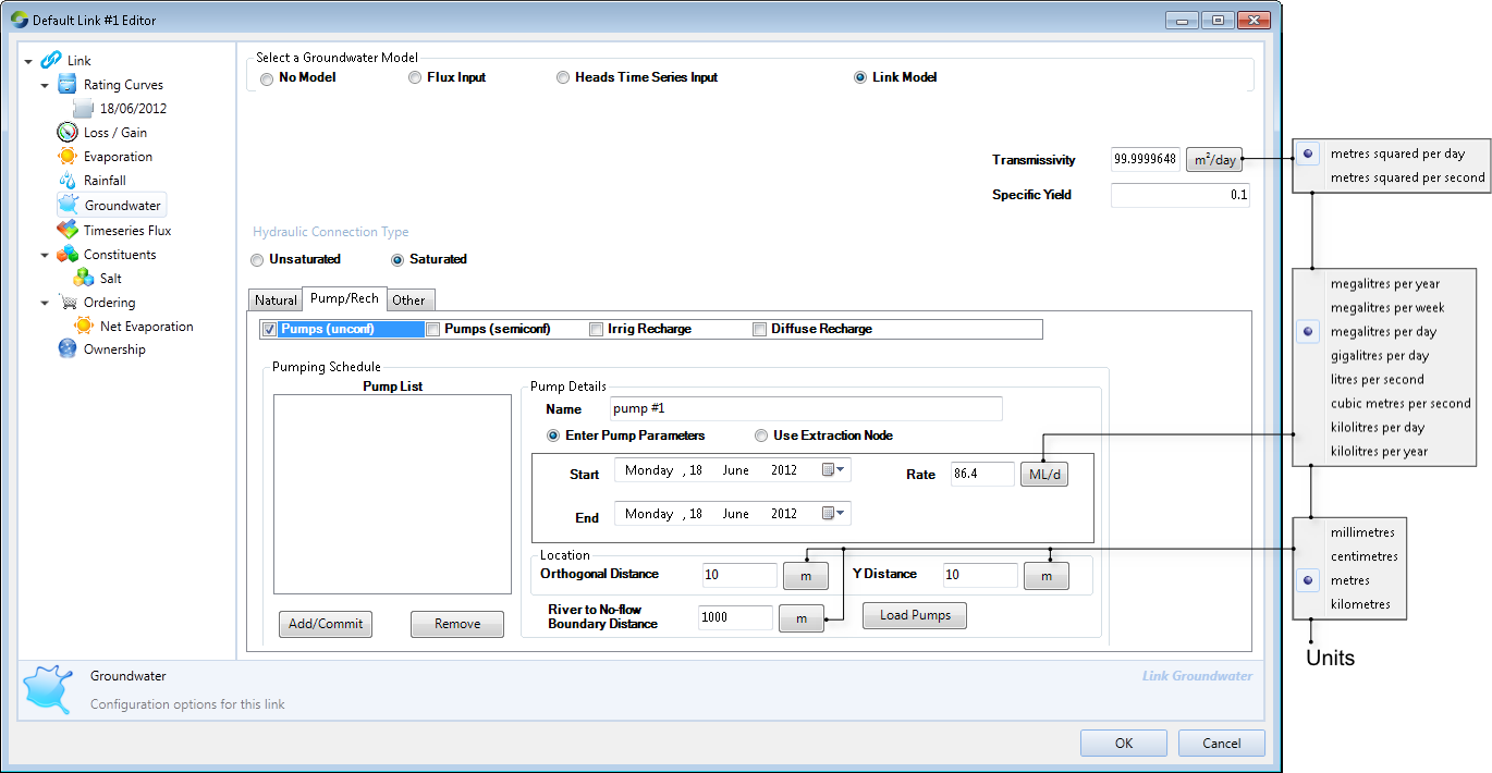
Figure 9. Link (Groundwater, saturated, irrigation recharge)
Irrigation recharge
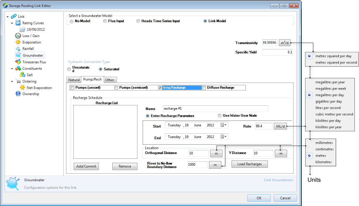
Irrigation recharge (Figure 10) works in a similar way as an unconfined aquifer except that, when recharge occurs, the cone of depression is inverted to form a groundwater mound, recharging the aquifer. If a sufficient groundwater head is developed the recharge water returns to the stream via aquifer discharge.
Since it is modelled in the same manner as pumping from an unconfined aquifer, they share similar parameters (with the exception that Pumping Rate is called Recharge Rate) and the controls for entering these parameters are almost identical. As with pumping, you can add irrigation recharge locations either manually or from a file.
Figure 10. Link (Groundwater, saturated, diffuse recharge)
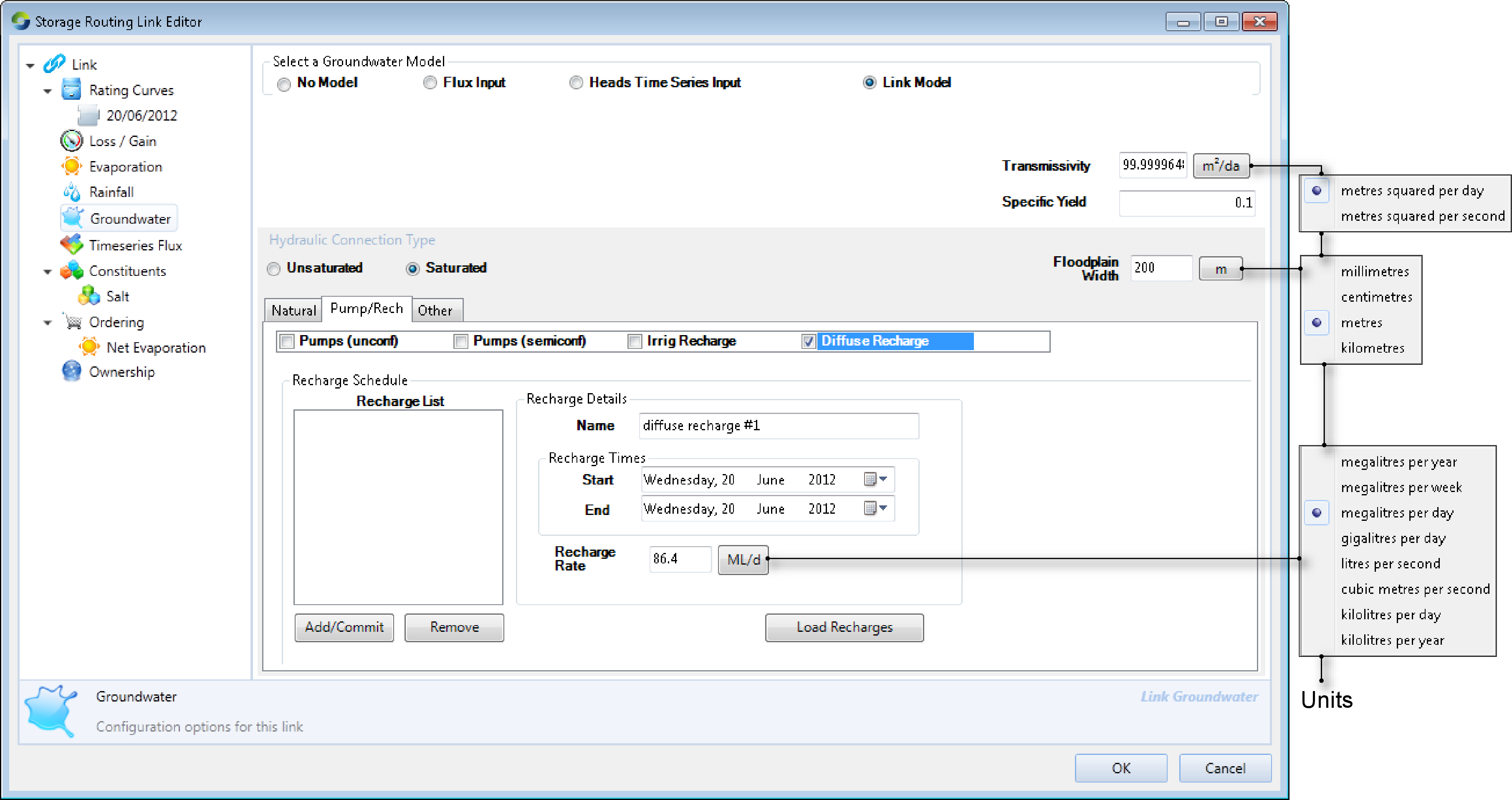
Unlike irrigation recharge which is applied at specific locations on the floodplain, diffuse recharge (Figure 11) is applied across the whole of the floodplain simultaneously. It infiltrates through the surface soil and recharges the aquifer, and if sufficient head difference is achieved, causes the aquifer to discharge water to the stream. The process model requires three shared aquifer parameters (Transmissivity, Specific yield and Floodplain width) and four process-specific unshared parameters:
- Name - a unique text string representing the pump name or number;
- Start time - the day on which the diffuse recharge commenced;
- End time - the last day of recharge; and
- Recharge rate.
Figure 11. Link (Groundwater, saturated, diffuse recharge)
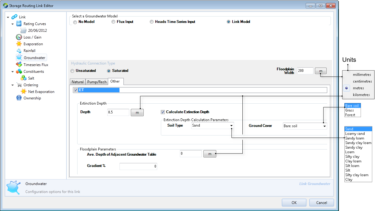
Evapo-transpiration
The Evapotranspiration process model (Figure 12) calculates the amount of water which is lost from the aquifer by evapotranspiration (ie plant transpiration and/or bare soil evaporation). The model requires Floodplain width as a shared aquifer parameter and three process specific unshared parameters:
- Extinction Depth - the depth to water table at which ET no longer happens;
- Average Depth of Adjacent Groundwater Table - the average depth of the water table; and
- Gradient - the hydraulic gradient of the aquifer as a percentage.
Groundwater evapotranspiration is assumed to decrease with increasing depth to water table and the extinction depth is the depth at which groundwater evapotranspiration attains a value of zero.
Figure 12. Link (Groundwater, saturated, ET)