Importing data

This section describes how to input data into Source. Any data pre-processing or similar is not discussed here. Click here to get an overview of these techniques.

Data input methods

Source allows you to load and manage all input data at a central location using the Data Sources Explorer. You can load data in the Explorer, edit it, and use it several times in the same model. There are two types of data input methods:

File - when uploading time-series files for any model, the data files do not always stipulate units. Select the appropriate units, as detailed in Time series; or
The output of a scenario - you can use the results of a previous run from a different scenario as an input to a run in the current scenario. Refer to Scenario linking for details.

When data (in the form of time series or a scenario) is added in the Data Sources Explorer, it is referred to as a data source and is available throughout Source and can be accessed in several ways:

In a feature editor - Figure 1. Inflow Node, Additional Flow shows an inflow node with data loaded from the Data Sources Explorer;
Using the Function Editor - reference a data source in a function or expression, such as if ($ACTIVE_DATA_SET == "Wet",5,10);
Using the command line runner (refer to Command Line Runner Options for details on how to reference it); or
Output of the Climate Data Import tool - refer to /wiki/spaces/SD35/pages/57872292.

Note: Data sources are scenario-specific. If you want to use a data source in two scenarios, you must load them individually for each scenario.

Input sets

In Source, an input set consists of a group of data sources that can be used to represent a weather feature, for example. You can switch between different input sets to compare the effects on a model. For example, you can have one input for natural conditions, another for wet conditions and a third set for dry conditions. Input sets allow you to easily keep the model structure, while changing the input data.

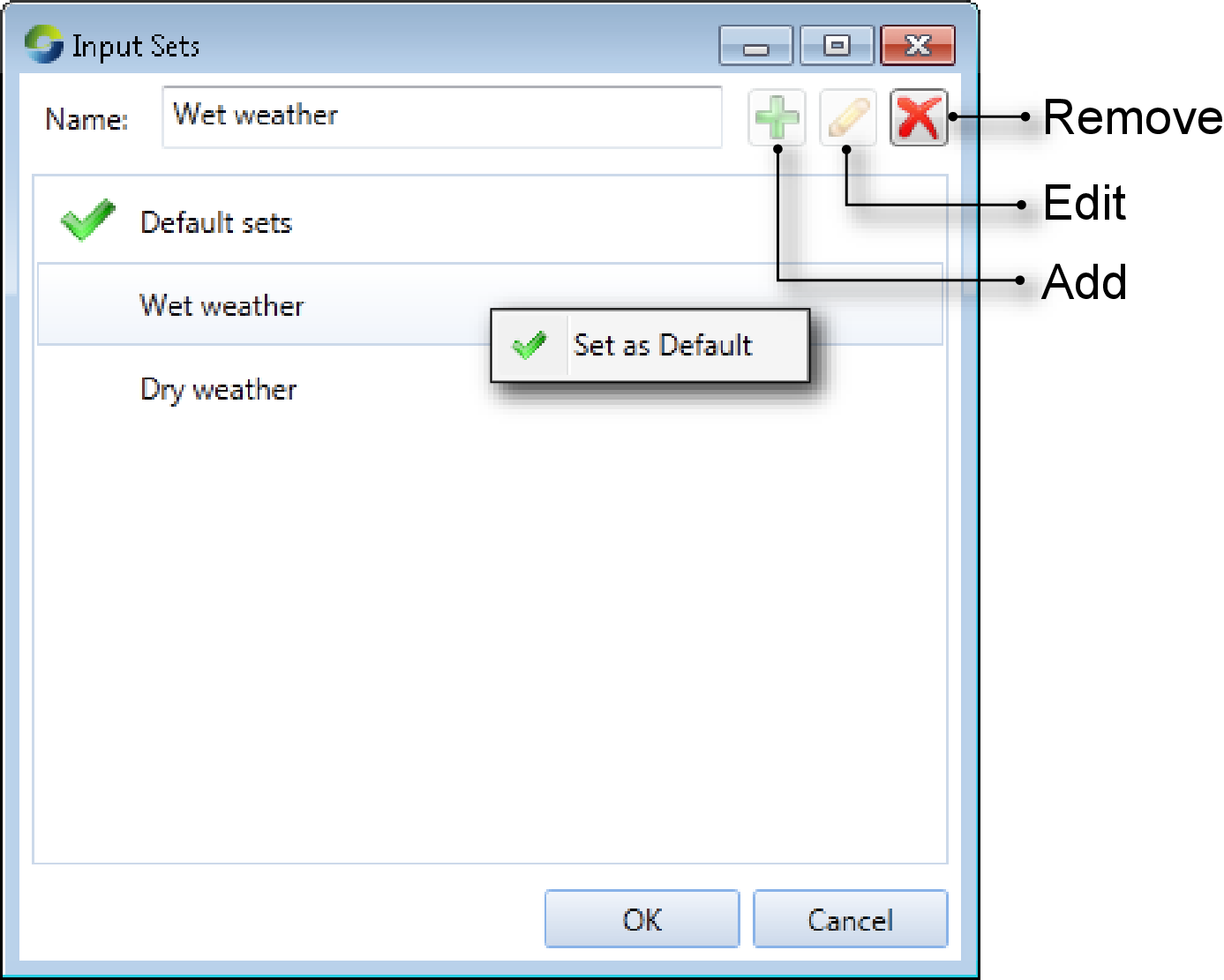
Choose Edit > Input Sets... to open the Input Sets dialog (Figure 1). You can manage them as follows:

To add an input set, enter its name in the Name field and click Add;
To change the name of an input set, choose the input set from the list, then enter the new name in the Name field and click Edit; or
To remove an input set, choose it from the list, then click Remove.

Figure 1. Input Sets

About "Reload on Run"

In many cases, there is a Reload on Run checkbox associated with the controls for loading data into Source. Regardless of whether the data source is a file or another scenario, it is loaded into an internal store.

If Reload on Run is turned off, Source will use a copy of the data present in its internal store until you either:

Turn on Reload on Run; or
Click Load and designate a data source (either the same file or a new one).

If Reload on Run is enabled, Source will reload its internal store from the original source each time you click the Begin Analysis (Run) button. In other words, if Reload on Run is turned off and you change the source file, Source will continue to use the data in its internal store.

Conversely, if Reload on Run is turned on and you change the source data, Source will update its internal store each time you run the model. The corollary is that you must ensure that your data sources are accessible for every run.

Loading data

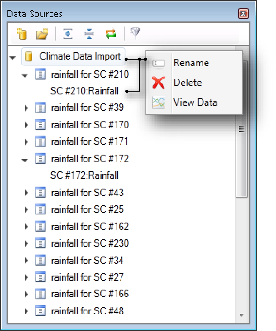
You can associate data with an input set in the Data Sources Explorer or in a node or link’s feature editor. Figure 2 shows features of the Explorer containing all data sources available in the scenario, both from time series files and scenarios. Additionally, it shows the nodes that each data source is associated with.

Figure 2. Data Sources Explorer

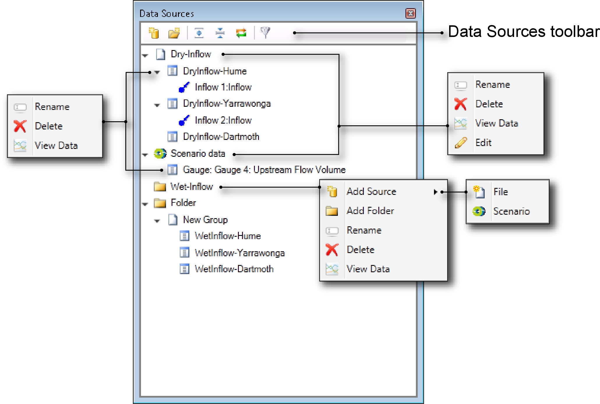
In each of the contextual menus, View Data opens the time series in the charting tool and Edit allows you to change the data source.

Time series

Open Figure 3 as follows. Either:

Click the New Data Source... button on the Data Sources toolbar and choose File Data Source from the drop down menu; or
Click File on the Data Sources toolbar. Then right click on the Folder icon and choose Add Source > File from the contextual menu.

Figure 3. New Data Source, Time series

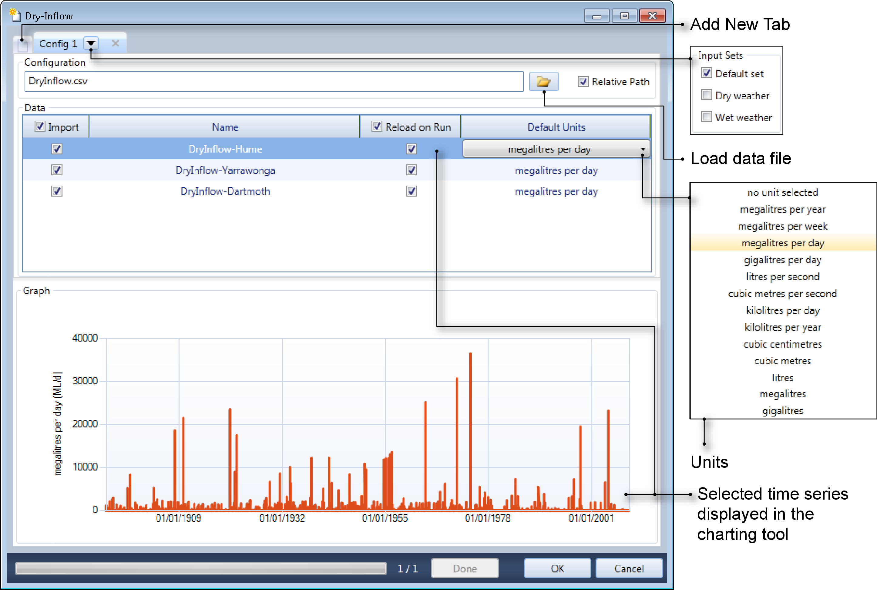
To load a time time series:

Click the Load data file icon and load the required time series;
Each column in the time series represents a row in the Data table. Click on the Default Units cell and choose the appropriate units from the drop down menu.
You can also choose which input set the time series will be associated with by clicking on the arrow for the Config 1 tab; and
If you enable the Relative Path check box, the paths displayed is the location of the time-series file relative to the project. Note that the project must have been saved prior to this.

Note: It is imperative that you specify compatible units for a time series after loading. If you do not, the time series will either not display in the Data Sources Explorer of the node’s feature editor or will provide incorrect results. You also need to view the time series in the chart view to complete the load process.

To disconnect a time series from a node or link, open the required feature editor. In the Data Sources Explorer, click on the Group that contains the file. The time series will be removed from the node. This can be confirmed by checking the Data Sources Explorer in the main screen.

Scenario linking

To link to the output of a scenario, click the Scenario Data Source... button on the Data Sources toolbar and choose Scenario Data Source from the drop down menu or click File on the Data Sources toolbar. Then right click on the Folder icon and choose Add Source » Scenario from the contextual menu. This opens the New Group dialog (shown in Figure 4).

Figure 4. New Data Source, Scenario Linking

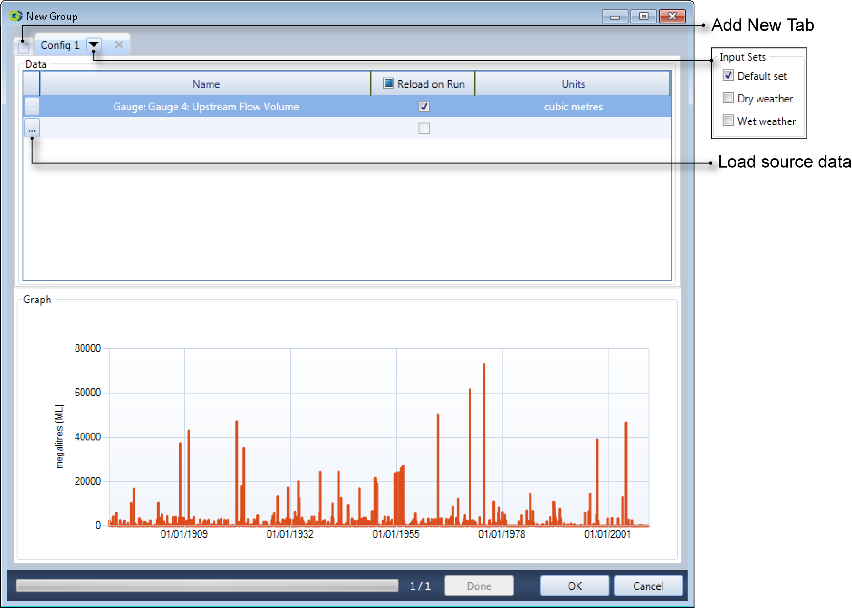
Note: You can only link to the result of a scenario run. Therefore, ensure that the other scenario has been run before you create the link.

To add a scenario as a data source:

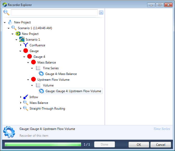
Click on the ellipsis button on the first column of the Data table (Load source data), which opens the Recorder Explorer (Figure 5);
This dialog lists the attributes that have been recorded for all the nodes and links in the scenario. Choose the attribute that you wish to use as input data to another scenario. In Figure 5, this data is the Upstream Flow Volume attribute;
Click OK to close the Recorder Explorer;
The New Group dialog now shows the Upstream Flow Volume in the Name column. If required, enable the Reload on Run checkbox;
The units are set automatically from the recorder chosen;
Just as with time series, you can the input set that is associated with this data source; and
To load another scenario data source, repeat this process.

Figure 5. New Data Source, Recorder Explorer

An extended discussion on data file formats begins at File formats later in this chapter. The ASCII file formats supported by Source are summarised in Table 5, Table 6 and Table 7.

Data from Import tool

Refer to /wiki/spaces/SD35/pages/57872292 for generating data. Once the tool has imported data, it can be used as a data source. Figure 6 shows the Data Sources Explorer with data generated by the tool, which can now be used as a time series.

Figure 6. Data Source Explorer, Climate Data Import

General requirements for data

Input data is specific to the component models that you use, but typically consists of climate, topography, land use, rainfall, and management practices. Examples are given in Table 1 and Table 2.

Table 1. Model calibration and validation (required data sets)

Base layers &
data

Common data
formats

Description and use

Observed flow
data preferably
at the same
time-step as
model

Time-series

Typically, you can use daily time-step gauging station data (ML/day or
m³/s) in the hydrologic calibration/validation process, or as a substitute
for modelled runoff as an observed flow time series at relevant nodes.
You need to assess the length of time for which records are available,
data quality and data gaps to determine how useful the data sets are for
calibration/validation. It is preferable to have data sets that are at least
10 years in duration and that cover both wet and dry periods.

When extracting gauged flow time-series data from databases
such as HYDSTRA (commercial software used across Australia for
archiving of gauge data), it is important to align the time bases for flow
with other climate data sets. For example, SILO data is collected each
day at 09:00 am, so each data point is the total rainfall for the previous
day. Therefore, when extracting flow data from HYDSTRA, ensure that
the “end of day” option is selected, so that the flow data will align with
the SILO rainfall data.
It is important to understand the conventions used by your organisation
as well as those that send you data - they may not be the same!

Observed water
quality data

Time-series

Data used in the water quality calibration/validation process. You need
to assess the length of time for which records are available, data quality
and data gaps to determine how useful the data sets are for calibration/
validation. It is preferable to have data sets that cover both storm event
and ambient conditions that include both wet and dry periods.

Existing reports

Report or
spreadsheet

Existing reports for the region may assist in hydrology and water quality
calibration process, eg load estimation.

Table 2. Optional data sets

Optional data sets	Common data formats	Description and use
Visualisation layers (eg roads, towns, soils, streams)	Polygons, polylines or points	You can add (drag and drop) additional layers into the Layer Manager and turn these layers on or off as required. These layers are not used in model development and are more a visualisation tool. The layers need to have the same projection and resolution as the DEM or sub-catchment map (but can have different extents).
Aerial & satellite imagery	Image	You can use aerial or satellite imagery to ensure the node-link network generated (either drawn manually or generated by Source) is correct. You can also use imagery to check the accuracy of the DEM-generated sub-catchment map. The layers need to have the same projection and resolution as the DEM or sub-catchment map (but can have different extents).
Local or relevant data on best management practices	Reports or spreadsheets	This includes information on locally-relevant best management practices that could be used when creating scenarios.
Existing hydrology and water quality reports and data	Relevant format	Existing reports for the region may help when you parameterise water quality models e.g EMC/DWC derivation. For example, an existing IQQM model of a region that uses the Sacramento rainfall-runoff model can be used to parameterise a Sacramento model in Source. Climate data sets may be used to speed up calibration of rainfall runoff models.

Note that all spatial data must use the same supported projections:

Albers Equal Area Comical;
Lambert Conic Conformal; or
Universal Transverse Mercator (UTM);

The exception is SILO gridded climate data, which is formatted in a geographic coordinate system.

Table 3 summarises the minimum necessary and optional input data needed to create a catchment model using Source.

Table 3. Building models (required data sets)

Base layers & data	Common data formats	Description and use
Digital Elevation Model (DEM)	Grid	A pit-filled DEM is used to compute sub-catchment boundaries and node-link networks. Source can automatically generate sub-catchment boundaries according to a user specified minimum drainage area (stream threshold) and flow gauging station positions. Selecting a small minimum sub-catchment area value will generate a large number of sub-catchments. This will increase the size of the project and run time.
Sub-catchment map	Grid	A sub-catchment map can be used in place of a DEM. This defines the sub-catchment boundaries within Source. You then need to draw the node-link network for the catchment.
Functional Unit (FU) map	Grid	A functional unit (FU) map divides the sub-catchments into areas of similar hydrological behaviour or response (eg land use). Source uses FU maps to assign functional unit areas. The FU map needs to have the same projection and resolution as the DEM or sub-catchment map (but it can have different extents provided the FU map at least covers the extent of the sub-catchments defined by the modeller).
Gauging station nodes	Point	Optionally, a shape file or ASCII text file that lists the gauging station coordinates, and an identifier such as gauge name or number that is used to define gauging station nodes. The coordinates of the gauges need to be in the same projection as the DEM or sub-catchment map. Incorporating the location of gauging stations as nodes can be particularly useful when calibrating the rainfall runoff model at a gauge.
Rainfall and PET data	Grid or time-series	Rainfall and potential evapotranspiration (PET) time series are used as inputs to the rainfall-runoff models. The most commonly-used files are SILO daily rainfall and PET ASCII grids. Using a daily ASCII grid format allows you to update the rainfall data at a later stage and re-run the model. Table 39 shows the format of the input data required. If local data is available, you can also attach your own rainfall data files to rainfall runoff models for each FU within a sub-catchment.
Point source data (if storages are to be modelled)	Time series	Outflow and/or constituent data. The time-series needs to have the same time-step, and should be run for at least the same duration, as the climate or flow inputs to the model.
Storage details (if storages are to be modelled)	Time series	Includes coordinates, maximum storage volume, depth/surface area volume relationship, observed inflow and outflow data, losses, extractions, release rules, dam specifications, gates, valves, etc.
Stream Network layer (optional)	Polyline	A stream network layer ensures the node-link network you build over the sub-catchment map is correct. You can then check the accuracy of the DEM-generated sub-catchment map.
USLE (Universal Soil Loss Equation) and or gully density layers (optional)	Grid	Can be used to spatially vary EMC/DWC values in the constituent generation process (use the Scale EMCs and DWCs using Hazard Map constituent generation method available through the Spatial data preprocessor plugin). The layers need to have the same projection and resolution as the DEM or sub-catchment map (but can have different extents).

Data formats

For gridded spatial data files, formats should be in ESRI text format (.ASC) or ESRI binary interchange (.FLT). Vector data should be in shape files. Gridded rainfall data can be ordered from either:

It is recommended that overlaying Digital Elevation Models (DEM), Functional units or sub-catchments have the same projection and resolution (but they can have different extents).

Zero-padded data

Certain file formats require data to be zero-padded. In Table 4, the first column represents months, and is not zero-padded. Some applications will sort this data as is shown in the second column. The third column is zero-padded and sorts correctly.

Table 4. Zero-padded data (sorting example)

Non-zero-padded data	Default sorting order	Zero-padding (always sorts correctly)
1	1	001
2	10	002
10	100	010
20	2	020
100	20	100
120	200	120

Times and Dates in data files

The TIME framework (used by Source) uses a subset of the ISO-8601 standard. The central part of this subset is the use of the format string:

yyyy-MM-ddTHH:mm:ss

Note: Microsoft Excel does not detect dates with the T symbol between the date and time. ISO-8601 permits replacing it with a space for the purposes of interchanging data and Excel will recognise that representation regardless of your regional and language settings.

Dates should comply with the ISO 8601 standard where possible but more compact formats will be read if unambiguous. For example:

the dates 24/01/2000 (Australian) and 01/24/2000 (USA) are unambiguous; but
the date 2/01/2000 is ambiguous and depends on the local culture settings of the host machine.

The TIME framework will always write dates in the following format:

yyyy-MM-dd

and it is recommended that you follow the same format and use zero padding within dates. For example, "2000-01-02" is preferred over "2000-1-1" to avoid ambiguity.

Annual data can often be entered by omitting a day number and using month number 01 (eg 01/1995; 01/1996).

Where a date-time specifier only contains a date, the reading is assumed to have occurred at time 00:00:00.0 on that date.

The smallest time-step that Source can currently handle is one second. When reading a data file, Source examines the first few lines to detect the date-time format and time-step of the time series:

If the format is ISO 8601 compliant, this format will be used to read all subsequent dates;
Failing that, an attempt is made to detect the dates and time-step with English-Australia ("en-AU") settings, for backward-compatibility reasons; and
Last, the computer configuration is used for regional and language settings.

Note: Data file format issues are often the result of incorrectly-formatted date and/or time entries. Refer to Data file formats (dates and time) for more details.

Predicted or calculated data

The predictions produced by an integrated model developed with Source depend on the selected component models. Example outputs include flow and constituent loads as a time series.

Missing entries

Missing entries are usually specified as -9999. Empty strings or white space are usually also read as missing values. Occasionally, other sentinel values are used, such as "-1?" in IQQM files.

Decimal points

Always use a period (".", ASCII 0x2E) as a decimal separator for numerical values, irrespective of the local culture/language/locale settings for Windows.

File formats

This section provides an overview of the file formats supported by Source. Table 5 lists the supported time-series data file formats. Raster data file formats are listed in Table 6. Several GIS, graphics and other formats that are also recognised by Source are listed in Table 7 but are not otherwise described in this guide

Table 5. Text-based time-series data file formats

File extension	Description
.AR1	Annual stochastic time series
.AWB	AWBM daily time series
.BSB	SWAT BSB time series
.BSM	BoM 6 minute time series
.CDT	Comma delimited time series
.CSV	Comma-separated value
.DAT	F.Chiew time series
.IQQM	IQQM time series
.MRF	MFM monthly rainfall files
.PCP	SWAT daily time series
.SDT	Space delimited time series
.SILO5	SILO 5 time series
.SILO8	SILO 8 time series
.TTS	Tarsier daily time series

Table 6. Text-based raster data file formats

File extension	Description
.ASC*	ESRI ASCII grids
.MWASC	Map window ASCII grids
.TAPESG	Grid-based Terrain Analysis Data

*GDAL compatible formats

Table 7. Other supported file formats

File extension	Description
.FLT	ESRI Binary Raster Interchange format
.JPG	GEO JPG Image (also .JPEG), and must have an associated .jgw world file
.MIF	MapInfo Interchange
.SHP*	ESRI Shape files (see )
.TIF*	GeoTIFF Image (also .TIFF)
.TILE	Tiled Raster Files
.TNE	Tarsier Node Link Network Files
.TRA	Tarsier Raster Files
.TSD	Tarsier Sites Data Files
.ADF*	ArcINFO/ESRI Binary Grid
.IMG*	ERDAS Imagine

*GDAL compatible formats

Annual stochastic time series

The .AR1 format contains replicates of annual time-series data generated using the AR(1) stochastic method. The file format is shown in Table 8. This format is not the same as the AR(1) format (.GEN) generated and exported by the Stochastic Climate Library.

Table 8. AR1 data file format

Row	Column (space-separated)
Row	1	2	3..nypr
1	desc
2	nypr	nr
odd	rn
even	value	value	value

Where: desc is a title describing the collection site

nypr is the number of years per replicate
nr is the number of replicates
rn is the replicate number in the range 1..nr
value is one of nypr data points per row for the replicate, to three decimal places.

ESRI ASCII grids

The .ASC format is a space delimited grid file, with a 6 line header as shown in Table 9. Values are not case sensitive and arranged in space delimited rows and columns, reflecting the structure of the grid. Units for cell size length depend on the input data, and could be either geographic (eg degrees) or projected (eg metres, kilometres). Units are generally determined by the application, with metres (m) being common for most TIME-based applications. For a file format description, refer to:

http://resources.esri.com/help/9.3/arcgisengine/com_cpp/gp_toolref/spatial_analyst_tools/esri_ascii_raster_format.htm

Arcinfo grid coverages can be converted to .ASC files using ESRI’s GRIDASCII command. ASC files can be imported into ArcGIS using the ASCIIGRID command.

Table 9. .ASC data file format

Row	Column (space-delimited)
Row	1	2	3..n
1	ncols	nc
2	nrows	nr
3	xref	x
4	yref	y
5	cellsize	size
6	nodata_value	sentinel
7..n	value	value	value

Where: nc is the number of columns

nr is the number of rows
xref is either XLLCENTER (centre of the grid) or XLLCORNER (lower left corner of grid)
yref is either YLLCENTER (centre of the grid) or YLLCORNER (lower left corner of grid)
(x,y) are the coordinates of the origin (by centre or lower left corner of the grid)
size is the cell side length
sentinel is a null data string (eg -9999)
value is a data point. There should be nc × nr data points.

AWBM daily time series

An AWBM daily time-series format file (.AWB) is an ASCII text file containing daily time-series data formatted as shown in Table 10. Dates (the year and month) were optional in the original AWBM file format, but are not optional in the format used in Source.

Table 10. AWB data file format

Row	Column (space-separated)
Row	1	2..ndays+1	ndays+2	ndays+3
1..n	ndays	value	year	month

Where: ndays is the number of days in the month (28..31)

value is the data point corresponding with a given day in the month (ie. ndays columns)
year is the year of observation (four digits)
month is the month of observation (one or two digits).

SWAT BSB time series

A .BSB is a line-based fixed-format file, typically used by applications written in FORTRAN. The header line gives the fields for the file with subsequent lines providing data for each basin to be used for each time-step. The format is shown in Table 11. For more details refer to the SWAT manual.

Table 11. .BSB data file format

Row	Character Positions (space padded)
Row	1..8	10..12	14..21	23..36	38..46
1	SUB	GIS	MON	AREAkm2	PRECIPmm
2..n	id	gis	mon	area	precip

Where: id is the basin identifier (both SUB and the id are text, left-aligned)

gis unknown (integer, right-aligned, eg. "1")
year unknown (integer, right-aligned, eg. "0")
area is the basin area in square kilometers (real, right aligned, eg "1.14170E+02")
precip is the basin precipitation in millimetres (real, right aligned, eg "1.2000").

BoM 6 minute time series

A .BSM (also .PLUV) is a fixed-format file, typically supplied by the Australian Bureau of Meteorology for 6 minute pluviograph data. The file has two header lines (record types 1 and 2) followed by an arbitrary number of records of type 3. The formats of record types 1..3 are shown in Table 12, Table 13 and Table 14, respectively.

All fields in .BSM files use fixed spacing when supplied, but Source can also read spaced-separated values.

Rainfall data points:

Each row of data contains all of the observations for that day.
The number of observations for a day depends on the observation interval. For example, if the observation interval is 6 minutes, there will be 24×60÷6=240 observations (raini fields) in each row of data.
Each raini field is in FORTRAN format F7.1 (a field width of seven bytes with one decimal place).
Assuming that observations are numbered from 1..n, the starting column position of any given raini field can be computed from 14+7×i
The unit of measurement is tenths of a millimetre (eg a rainfall of 2 mm will be encoded as "20.0").
Values are interpreted as follows:
0.0 means there was no rain during the interval.
a positive non-zero value is the observed rainfall, in tenths of a millimetre, during the interval.
If there is zero rain for the whole day, no record is written for that day.

Missing data:

A sentinel value of -9999.0 means that no data is available for that interval.
A sentinel value of -8888.0 means that rain may have fallen during the interval but the total is known only for a period of several intervals. This total is entered as a negative value in the last interval of the accumulated period. For example, the following the following pattern would show that a total of 2 millimetres of rain fell at some time during an 18-minute period:

-8888.0-8888.0 -20.0

If an entire month of data is missing, either no records are written or days filled with missing values (-9999.0) are written. No attempt is made to write dummy records if complete years of data are missing.

Example file

61078 1

61078 2 WILLIAMTOWN RAAF

61078 19521231 .0 .0 .0 [etc., 240 values]

61078 1953 1 1 .0 .0 .0 [etc., 240 values]

61078 1953 1 3 .0 .2 .0 [etc., 240 values]

61078 1953 115 .0 .0 .2 [etc., 240 values]

61078 1953 118 .0 .0 .0 [etc., 240 values]

61078 1953 212 .0 .0 .0 [etc., 240 values]

61078 1953 213 .0 .0 .0 [etc., 240 values]

61078 1953 214 .0 .0 .0 [etc., 240 values]

61078 19521231 .0 .0 .0 [etc., 240 values]

The following notes are taken from Bureau of Meteorology advice:

All data available in the computer archive are provided. However very few sites have uninterrupted historical record, with no gaps. Such gaps or missing data may be due to many reasons from illness of the observer to a broken instrument. A site may have been closed, reopened, upgraded or downgraded during its existence, possibly causing breaks in the record of any particular element.
Final quality control for any element usually occurs once the manuscript records have been received and processed, which may be 6-12 weeks after the end of the month. Thus quality-controlled data will not normally be available immediately, in "real time".

Table 12 .BSM data file format (record type 1)

Row	Character Positions (space padded)
Row	1..6	7..15	16	17..n
1..n	snum	blank	1	blank

Where: snum is the station number

blank ASCII space characters.

Table 13 .BSM data file format (record type 2)

Row	Character Positions (space padded)
Row	1..6	7..15	16	17..20	21..54	55..n
1..n	snum	blank	2	blank	sname	blank

Where: snum is the station number

sname is the station name
blank ASCII space characters.

Table 14 .BSM data file format (record type 3)

Row	Character Positions (space padded)
Row	1..6	7..12	13..16	17..18	19..20	21..n
1..n	snum	blank	year	month	day	{rain_i ...}

Where: snum is the station number

blank ASCII space characters
year is the year of the observation (four digits)
month is the month of the observation (one or two digits, right-aligned, space padded)
day is the date of the observation (one or two digits, right-aligned, space padded)
rain_i is a rainfall data point as explained below.

Comma delimited time series

A .CDT comma delimited time-series format file is an ASCII text file that contains regular (periodic) time-series data. The file type commonly has no header line but, if required, it can support a single line header of "Date,Time series 1".

You can use the .CDT format to associate observations with a variety of time interval specifications. Table 15 shows how to structure annual data, Table 16 how to specify daily data aggregated at the monthly level, and Table 17 the more traditional daily time series (one date, one observation). Table 18 explains how to supply data in six-minute format.

Table 15 .CDT data file format (annual time series)

Row	Column (comma-separated)
Row	1	2
1..n	year	value..n

Where: year is the year of observation (four digits, eg. 2011)

value is the observed value (eg 9876).

Table 16 .CDT data file format (time series with monthly data)

Row	Column (comma-separated)
Row	1	2..n
1..n	mm/yyyy	value

Where: mm is the month of observation (two digits, eg. 09)

yyyy is the year of observation (four digits, eg. 2011)
value is the observed value (eg. 2600).

Table 17 .CDT data file format (daily time series with daily data)

Row	Column (comma-separated)
Row	1	2..n
1..n	date	value

Where: date is the date of observation in ISO format (eg. 2000-12-31)

value is the observed value (eg. 2600).

Table 18 .CDT data file format (six-minute time series)

Row	Column (comma-separated)
Row	1	2	3..n
1..n	date	time	value

Where: date is the date of observation in ISO format (eg 2000-12-31)
time is the time of observation in hours and minutes (eg 23:48)
value is the observed value (eg 10).

Comma-separated value

A comma separated value or .CSV file is an ASCII text file that contains data in a variety of representations. When a .CSV contains regular (periodic) time-series data, there are at least two columns of data. The first contains a time-stamp and the remaining columns contain data points associated with the time-stamp. The format is shown in Table 19. All columns are separated using commas. Annual data can be entered using the notation 01/yyyy where yyyy is a year. Header lines in .CSV files are usually optional.

Table 19 .CSV data file format

Row	Column (comma separated)
Row	1	2..n
1	Date	desc
2..n	date	value

Where: desc is a title for the column (header rows are often optional).

date is a date in ISO 8601 format ("yyyy-MM-dd HH:mm:ss" where " HH:mm:ss" is optional)
value is a data point (eg a real number with one decimal place).

F.Chiew time series

A .DAT is a two-column daily time-series file with the fixed format shown in Table 20. Note that the first two characters in each line are always spaces with the data starting at the third character position.

Table 20 .DAT data file format

Row	Character Positions (space padded)
Row	1..2	3..6	7..8	9..10	12..20
1..n	blank	year	month	day	value

Where: blank ASCII space characters

year is the year of the observation (four digits)
month is the month of the observation (one or two digits, right-aligned, space padded)
day is the date of the observation (one or two digits, right-aligned, space padded)
value is the data point (real, two decimal places, right aligned, eg "1.20").

IQQM time series

An .IQQM time-series format file is an ASCII text file that contains daily, monthly or annual time-series data. The file has a five line header formatted as shown in Table 21. The header is followed by as many tables as are needed to describe the range delimited by fdate..ldate. The format of each table is shown in Table 22.

Each value is right-justified in 7 character positions with one leading space and one trailing quality indicator. In other words, there are five character positions for digits which are space-filled and right-aligned. The first value in each row (ie the observation for the first day of the month) occupies character positions 5..11. The second value occupies character positions 12..18, the third value positions 19..25, and so on across the row. In months with 31 days, the final value occupies character positions 215..221. The character positions corresponding with non-existent days in a given month are entirely blank. The mtotal and ytotal fields can support up to 8 digits. Both are space-filled, right-aligned in character positions 223..230.

The quality indicators defined by IQQM are summarised in Table 23. At present, Source does not act on these quality indicators.

Missing data points are generally represented as "-1?". A value is also considered to be a missing data point if it is expressed as a negative number and is not followed by either an "n" or "N" quality indicator.

Divider lines consist of ASCII hyphens (0x2D), beginning in character position 5 and ending at position 231.

Example file

Title: Meaningful title     Date:06/08/2001 Time:11:38:25.51
Site : Dead Politically Correct Person's Creek
Type : Flow
Units: ML/d
Date : 01/01/1898 to 30/06/1998      Interval : Daily
Year:1898
     ------------------------------------ ------------------------------------
       01    02    03    04   05    06  ...  28    29    30    31     Total
     ------------------------------------ ------------------------------------
Jan    3     4     3     4    3      4        2    3     2     3       224
Feb    2     3     2     3    2      3        2                        134
Mar    3     22    4     2    2      2        1    2     1     2       84
Apr    1     2     1     2    1      2        1    1     1             37
May    1     1     4     3    53     33       1    1     1     1       143
Jun    1     1     0     1   -1?     7        63   58    52            816
Jul    48    43    40    36   33     30       77   70    63    59      1389
Aug    54    49    46    41   39     35       30   28    26    420     2433
Sep   880   362   282   256  245     215      241  39    36            4414
Oct    35    33    31    31   29     28       22   28    20    17      783
Nov    15    16    15    18   16     15       11   12    11            415
Dec    12    11    11    11   11     10       9     8    9     8       422
----------------------------------------- ------------------------------------
                                                                       11294

Table 21 .IQQM data file format (header part)

Row	Character Range	Key	Character Range	Value
1	1..6	Title:	8..47	title
	54..58	Date:	59..68	cdate
	71..75	Time:	76..86	ctime
2	1..6	Site :	8..47	site
3	1..6	Type :	8..22	type
4	1..6	Units :	8..17	units
5	1..6	Date :	8..17	fdate
	19..20	to	22.31	ldate
	36..45	Interval :	47..n	interval
6	<<blank line>>

Where: title is a string describing the file’s contents

cdate is the date on which the time series was created (dd/mm/yyyy)
ctime is the time on cdate when the time series was created (hh:mm:ss.ms)
site is a string describing the measurement site
type is a string specifying the data type (eg. precipitation, evaporation, gauged flow)
units is a string specifying the units of data (eg. mm, mm*0.1, ML/day)
fdate is the first date in the time series (dd/mm/yyyy)
ldate is the last date in the time series (dd/mm/yyyy)
interval is a string defining the collection interval (eg. daily, monthly)

Table 22 .IQQM data file format (table part)

Row	Logical column (fixed width)
Row	1	2..13	14
+0	Year:year Factor= factor
+1	<<divider line>>
+2		dd	Total
+3	<<divider line>>
+4..+15	mmm	value	mtotal
+16	<<divider line>>
+17			ytotal
+18	<<divider line>>

Where: year defines the year implied for the following table (yyyy)

factor if present, each value in the table is multiplied by factor (if omitted, the default is 1.0)
dd is the day of the month from 01..31 (zero-padded)
mmm is the first three characters of the name of the month (eg Jan, Feb)
value is a data point. There should be as many data points in the row as the month has days
mtotal is the sum of the daily values in the month
ytotal is the sum of the monthly values in the year.

Table 23 .IQQM data file format (quality indicators)

Character	Interpretation
" " (space)	Accept value as is
"*"	Multiply value by +1,000.0
"e"	The value is only an estimate
"E"	The value is only an estimate but it should be multiplied by 1,000
"n"	Multiply value by -1.0
"N"	Multiply value by -1,000.0
"?"	Missing data indication (typically input as "-1?")

MFM monthly rainfall files

A .MRF text file format contains a header line followed by a line giving the number of years of data. Data are formatted in lines with year given first, followed by 12 monthly values, all space separated. The format is shown in Table 24.

Table 24 .MRF data file format

Row	Column (space-delimited)
Row	1	2..13
1	desc
2	nyears
3..n	year	mvalue

Where: desc is a string describing the file’s contents (eg "Swiftflow River @ Wooden Bridge")

nyears states the number of years (rows) of data in the file
year is the year of observation (four digits)
mvalue is a data point. Each year should have 12 data points in the order January...December.

Map window ASCII grids

The .MWASC ASCII grid is similar to .ASC except that the coordinates are offset by 1/2 cell size and the header rows do not have titles. Thus there are six header rows with parameters only, followed by the gridded data. The format is shown in Table 25.

Table 25 .MWASC data file format

Row	Column (space-delimited)
Row	1	2..n
1	nc
2	nr
3	xc
4	yc
5	size
6	sentinel
7..n	value	value

Where: nc is the number of columns

nr is the number of rows
(xc,yc) are the coordinates of the center of the call at the lower left corner of the grid
size is the cell side length
sentinel is a null data string (eg -9999)
value is a data point. There should be nc × nr data points.

SWAT daily time series

A SWAT daily rainfall time-series format file (.PCP) is an ASCII text file that contains daily time-series rainfall data. The file has a four line header followed by daily data values as shown in Table 26.

Table 26 .PCP data file format

Row	Column (space-delimited)
Row	1	2
1	desc
2	Lati	lat
3	Long	lon
4	Elev	mahd
5..n	yyyydddvvv.v

Where: desc is a string describing the file’s contents (eg "Precipitation Input File")
lat is the latitude of the site in degrees (eg 14.77)
lon is the longitude of the site in degrees (eg 102.7)
mahd is the elevation of the site in metres (eg 167)
yyyy is the year
ddd is the Julian day offset within the year
vvv.v is the data value expressed as four digits with one decimal place.

Space delimited time series

A space- or tab-delimited (.SDT) column time-series format file is an ASCII text file that contains time-series data. There is no header line in the file. The format is shown in Table 27. Monthly and annual data can be entered using month and/or day number as 01. These files can be created in a spreadsheet application by saving correctly formatted columns to a text (.TXT) format.

Table 27 .SDT data file format

Row	Column (space- or tab-delimited)
Row	1	2	3	4
1..n	year	month	day	value

Where: year is the year of observation (four digits)

month is the month of observation (one or two digits)
day is the day of observation (one or two digits)
value is the data value to three decimal places (eg. 14.000).

SILO 5 time series

A QDNR .SILO5 daily time-series format file is an ASCII text file that contains daily time-series data. The format is shown in Table 28. This format sometimes uses the .TXT file extension.

Table 28 .SILO5 data file format

Row	Column (space-delimited)
Row	1	2	3	4	5
1..n	year	month	day	jday	value

Where: year is the year of observation (four digits)

month is the month of observation (one or two digits)
day is the day of observation (one or two digits)
jday is the Julian day offset within the year (one, two or three digits)
value is a data point.

SILO 8 time series

The .SILO8 format contains the full 8 column daily data set from the SILO data base. The file can have multiple header lines, enclosed in inverted commas. The format of data rows is shown in Table 29.

Table 29 .SILO8 data file format

Row	Column (space-delimited)
Row	1	2	3	4	5	6	7	8
1..n	maxt	mint	rain	evap	rad	vpress	maxrh	minrh

Where: maxt is the maximum temperature

mint is the minimum temperature
rain is the rainfall
evap is the evaporation
rad is the radiation
vpress is the vapour pressure
maxrh is the maximum relative humidity
minrh is the minimum relative humidity.

Grid-based Terrain Analysis Data

A .TAPESG file is a three column raster data format, with space separated values. Each line consists of the X coordinate, Y coordinate, and value. The format is shown in Table 30.

Table 30 .TAPESG data file format

Row	Column (space-delimited)
Row	1	2	3..n
1	x	y	value

Where: (x,y) are coordinates

value is a data point.

Tarsier daily time series

The Tarsier daily time-series format file (.TTS) is an ASCII text file that contains daily time-series data. The file has a 21-line header (Table 64) followed by daily data values in the format shown in Table 31.

Example file header

Tarsier modelling framework, Version 2.0.
:  Created by Fred Watson.
:  File Name : C:\data\TIME\TIMEExample.tts
:  Generated from TIME Framework
:  Date : 24/12/2004 11:59:30 PM
:  File class: TTimeSeriesData.
FileVersion unknown
HeaderLines 1
1.
NominalNumEntries 10
XLabel Date/Time
Y1Label Y1
Y2Label Y2
Units mm.day^-1
Format 1
Easting 0.000000
Northing 0.000000
Latitude 0.000000
Longitude 0.000000
Elevation 0.000000
*

Note: Source will warn you if you import data containing negative numbers. Also, the presence of any zero values in the data stream will hamper your ability to adjust the Y-axis to show log values in the Charting Tool.

Table 31 .TTS data file format

Row	Column (space-separated)
Row	1	2	3	4
1..21	header
22..n	year	jday	value	qual

Where: header is a 21-line header. Refer Table 32.

year is the year of observation (four digits)
jday is the Julian day offset within the year (one, two or three digits)
value is a data point including optional decimal places (eg 14 or 14.000)
qual is a quality indicator ("." ASCII 46 = "data ok/present"; "-" ASCII 45 = "data missing").

Table 32. Tarsier Daily Time Series

Line	Purpose
1	The Tarsier version number header
2	Reference to author of Tarsier modelling framework
3	File path and name
4	Name of software used to create the file
5	Date and time file was created
6	Tarsier timer series data class (eg TTimeSeriesData)
7	File version number
8	Number of header lines (set to 1)
9	1. (the number 1 followed by a period)
10	Number of daily data entries in the file
11	Xlabel is always Date/Time for time-series data
12	Y1Label Y1 fixed field, doesn’t change
13	Y2Label Y2 fixed field, doesn’t change
14	Units followed by Data units
15	Format followed by format information (eg 1)
16	Easting followed by grid position east in metres
17	Northing followed by grid position north in metres
18	Latitude followed by the latitude of the site in decimal degrees
19	Longitude followed by the longitude of the site in decimal degrees
20	Elevation followed by the elevation of the site in metres
21	Header character (usually an asterisk; ASCII 42, ASCII hex 2A)

Table 33. Climate data import tool (gridded data file formats)

Rainfall	PET
ASCIIGrids	ASCIIGrids
Climate Atlas of Australia	Climate Atlas of Australia
QDNR Silo	Silo 2006 standard
Silo 2006 standard	Silo Morton
Silo comma delimited
Silo Morton

Note: Before importing ASCIIGrid files that have been obtained from Silo at different times (eg. data for 1950-2004 obtained in 2005 and data for 2004-2007 obtained in 2007), refer to Climate data formats - ASCII Grids.

For Climate Atlas of Australia file types, see the Bureau of Meteorology’s web site:

http://www.bom.gov.au/climate/data/index.shtml

For QDNR Silo; Silo 2006 standard; Silo comma delimited; Silo Morton; Silo original standard see the Queensland Government Department of Environment and Resource management (QDERM) website:

http://www.longpaddock.qld.gov.au/silo/

CentralMeridian, FirstParallel, SecondParallel, OriginLatDD, OrginLongDD, EastFalseOrigin and NorthFalseOrigin are parameters to transform the Albers or Lambert projections of the scenario data into latitude and longitude co-ordinates of the climate ASCII grid data. They have been set to defaults for all of Australia and can be altered to better represent your modelling location. It is recommended that the Australian standard be adopted. Table 66 specifies the Albers projection parameter values for Australia and Queensland.

Table 34. Albers projection parameter values (Australia & QLD)

Field	Units	Australian Standard	Queensland ERA value
Projection		Albers	Albers
Central Meridian	Decimal degrees	132.0	146.0
First Parallel	Decimal degrees	-18.0	-13.1667
Second Parallel	Decimal degrees	-36.0	-25.8333
Origin Latitude	Decimal degrees	0.0	0.0
Origin Longitude	Decimal degrees	132.0	146.0
East False Origin	Meters	0.0	0.0
North False Origin	Meters	0.0	0.0

For importing all other file formats, only the Universal Transverse Mercator (UTM) Zone needs to be defined. The UTM is a geographic coordinate system that provides locations on the Earth’s surface. It divides the Earth into 60 zones, from West to East. Australia falls into zones 49-56. Refer to the Geosceience Australia website (www.ga.gov.au) for details about the UTM zones in Australia.

Climate data formats - ASCII Grids

The Climate Data Import Tool will import any grids that follow the ESRI ASCIIGrid format and are in latitude-longitude projection. Therefore, it replaces the need to use a large set of Data Drills (eg. 10,000) by importing ASCIIGrid files of the catchment directly. The main benefits of ASCIIGrids are that the files are smaller and easier to manage, and Silo can usually supply them more easily than thousands of Data Drills.

When using ASCIIGrids of PET from SILO for hydrological purposes, request daily MWet (Morton’s areal potential). If data is for agricultural purposes, request daily FAO56 (Penman-Monteith).

ASCIIGrid Advanced Example 1

Suppose you have data for one catchment and you want to use it to analyse a second catchment that is mostly in the same area, but with a small part that falls outside the available data.

In the example shown in Figure 7, the rectangle "a" indicates the area covered by the ASCIIGrid files. Shape "A" is the original catchment that the data was obtained for, and shape "C" is the catchment that you want to analyse. The problem is that part of "C" is outside of rectangle "a".

Providing that you are willing to accept that the results will be of lower quality, and also providing that no part of "C" is further than 10 kilometres from the boundary of "a" then the pre-processor will use the data from the nearest cell in "a" for the portion of "C" that is outside of "a". This is identical to the behaviour of the "Import rainfall data from SILO" option. To do this the prototypeRaster can be any raster (ASCIIGrid file) from "a".

Figure 7. Importing ASCIIGrid files (case 1)

ASCIIGrid Advanced Example 2

An additional set of data "b" that was used to analyse catchment "B" (Figure 8).

Grid "a" covers the period 1950-2004 and grids "b" covers the period 1987 to 2007. If you need to compare events in 2006-2007 for catchment "C" with the long term (50 years), you need to make use of data from both sets "a" and "b".

In this example the prototypeRaster should again be any raster from set "a". Note that by doing so the Climate Data Import Tool will again handle the small part of "C" that is outside of "a" in the same way as it did in Case 1, even when it is using data from "b". Therefore, if a small portion of a catchment is outside one set of grids then make your prototypeRaster one of that same set.

Data input methods

Input sets

Figure 1. Input Sets

About "Reload on Run"

Loading data

Figure 2. Data Sources Explorer

Time series

Figure 3. New Data Source, Time series

Scenario linking

Figure 4. New Data Source, Scenario Linking

Figure 5. New Data Source, Recorder Explorer

Data from Import tool

Figure 6. Data Source Explorer, Climate Data Import

General requirements for data

Table 1. Model calibration and validation (required data sets)

Table 2. Optional data sets

Table 3. Building models (required data sets)

Data formats

Zero-padded data

Table 4. Zero-padded data (sorting example)

Times and Dates in data files

Predicted or calculated data

Missing entries

Decimal points

File formats

Table 5. Text-based time-series data file formats

Table 6. Text-based raster data file formats

Table 7. Other supported file formats

Annual stochastic time series

Table 8. AR1 data file format

ESRI ASCII grids

Table 9. .ASC data file format

AWBM daily time series

Table 10. AWB data file format

SWAT BSB time series

Table 11. .BSB data file format

BoM 6 minute time series

Table 12 .BSM data file format (record type 1)

Table 13 .BSM data file format (record type 2)

Table 14 .BSM data file format (record type 3)

Comma delimited time series

Table 15 .CDT data file format (annual time series)

Table 16 .CDT data file format (time series with monthly data)

Table 17 .CDT data file format (daily time series with daily data)

Table 18 .CDT data file format (six-minute time series)

Comma-separated value

Table 19 .CSV data file format

F.Chiew time series

Table 20 .DAT data file format

IQQM time series

Table 22 .IQQM data file format (table part)

Table 23 .IQQM data file format (quality indicators)

MFM monthly rainfall files

Table 24 .MRF data file format

Map window ASCII grids

Table 25 .MWASC data file format

SWAT daily time series

Table 26 .PCP data file format

Space delimited time series

Table 27 .SDT data file format

SILO 5 time series

Table 28 .SILO5 data file format

SILO 8 time series

Table 29 .SILO8 data file format

Grid-based Terrain Analysis Data

Table 30 .TAPESG data file format

Tarsier daily time series

Table 31 .TTS data file format

Table 32. Tarsier Daily Time Series

Table 33. Climate data import tool (gridded data file formats)

Table 34. Albers projection parameter values (Australia & QLD)

Climate data formats - ASCII Grids

ASCIIGrid Advanced Example 1

Figure 7. Importing ASCIIGrid files (case 1)

ASCIIGrid Advanced Example 2

Figure 8. Importing ASCIIGrid files (case 2)