Ordering
Introduction
A regulated river system may be composed of several upstream reservoirs on multiple flow paths, thus providing a number of options to supply the downstream water order. During the ordering phase, water orders are accumulated from downstream to upstream and consider the average travel time, or order time of water (bound by the minimum and maximum travel time). Order time is calculated in the demand phase and is used to determine how many time-steps into the future water orders need to be processed for at each network component.
Orders can be processed in one of two ways:
- Rules-based ordering - Uses in-built rules which process the release of water; or
- Network Linear Programming (NetLP), also known as Multiple Supply Path (MSP) ordering - uses "linear programming" techniques to find optimal solutions. The term "linear programming" is often described as "planning with linear models" to avoid any confusion with the discipline of writing computer programs.
Take the following into consideration when deciding which type of ordering to configure for your scenario:
- Rules based ordering performs well for both daily and longer time-steps. A daily time-step may cause performance issues with optimised ordering, as the number of nodes in its solution network multiplies as the time-step reduces from monthly to daily unless travel times are short. Also, the optimised solution only considers inflows in the current time-step, so its solution may not be as efficient. If a longer time-step (such as monthly) is used, the optimised ordering system is likely to provide more efficient solutions than rules based ordering, with comparable performance;
- If you know about future inflow to and losses from the supply system, optimised ordering is a better solution as it provides a method of forecasting;
- If the rules that determine which supply path to use at various storage levels are well established, rules based ordering should be more efficient than optimised ordering; and
- Rules based ordering should be used if the objective of the scenario is to model what an operator does.
Enabling ordering
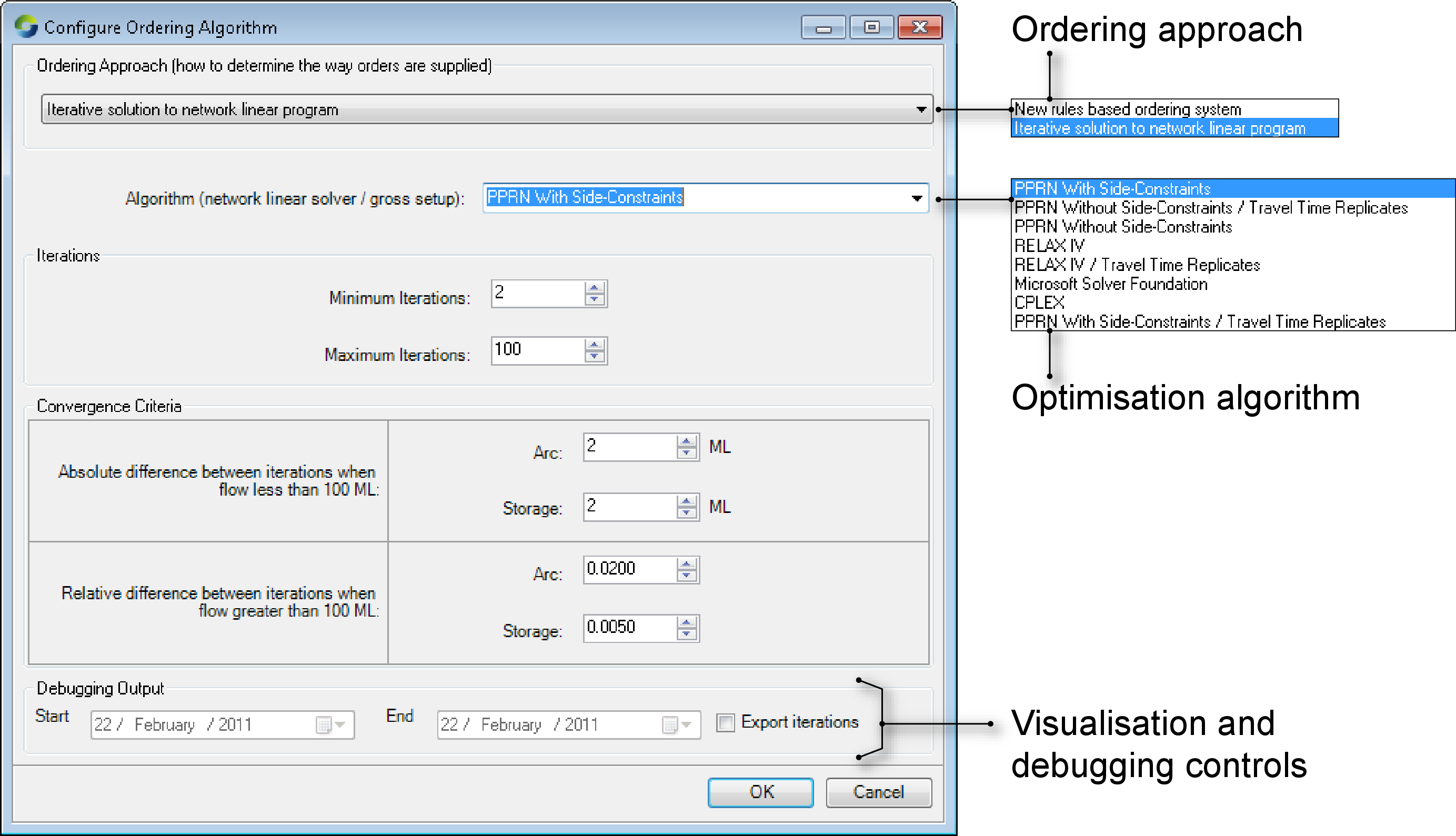
You must enable ordering prior to configuring the type of ordering. Begin by choosing or click Configure Ordering on the Ordering toolbar and choose Algorithm.... This opens the Configure Ordering Algorithm dialog (Figure 1). Choose New rules based ordering system from the Ordering Approach drop-down menu to configure rules-based ordering. For netLP, choose Iterative solution to network linear program.
Figure 1. Enabling ordering
Each node must be configured differently depending on the type of ordering methodology used. This chapter describes how to set up nodes for each method.
Rules-based ordering
There are two key components for rules-based ordering:
- Calculation of order time within a network - order time is calculated in the initialisation phase of a Source project and is required by the ordering and off-allocation systems to determine how many time-steps into the future water orders need to be processed for at each network component; and
- The way orders in the network are processed at each node/model component - Orders are processed in the constraint and order phases. During the ordering phase, water orders and off-allocation requests are accumulated from downstream to upstream and consider the average travel time of water in the regulated river system downstream of a reservoir.
Rules-based ordering at nodes and links
In the ordering phase, rules based ordering system calculates the total volume of order required at each node and link to meet downstream demand. Orders are received at a node from the downstream node, is adjusted as required, then passed upstream. The adjustment usually involves changing volumes ordered, but at some node types (splitter, confluence, storage) it also involves merging, splitting or resetting the order.
For example, assume an order reaching a loss node is 100ML, but due to its characteristics, it loses 20ML. To make up for this reduction, the loss node must now order 120ML, which is the new order that travels upstream. This section deals with processing of orders when ownership has not been enabled (ie. a system containing a single, default owner).
Ordering is configured at the confluence and storage nodes, as well as at a storage routing link.
Confluence node
Refer to the Confluence node for configuring ordering at this node. Orders are passed onto the branch depending on the following:
- If orders are directed to a particular storage along a branch, the confluence node will pass them up that branch; or
- If orders can be supplied along multiple paths or by multiple storages, orders can be distributed using either the Harmony-based or Constraint-based method (refer to Confluence node for details).
Storage node
Source forecasts the volume of water in storage at the end of the order period so that it can place orders to keep the storage volume within its optimal operating range. The following parameters can be configured:
- Pass Orders Through Storage - enabling this parameter will cause the node to disregard any losses or gains occuring at the node;
- Forecast Inflow - Calculates an estimate of forecast inflow from upstream (specified as an expression); and
- Forecast Daily Net Evaporation - Monthly net evaporation, which can be imported as a time series.
Link
Routed links may gain or lose water due to rainfall, evaporation and groundwater (seepage) as flow does not travel from one end to another instantaneously. You can choose which of these lateral fluxes the ordering system takes into account by enabling the relevant checkbox shown in the node’s feature editor (Figure 2). The data for each of the fluxes is taken from its corresponding item in the hierarchical list. For example, if you enable Use Loss/Gain, Source uses the table specified in Loss/Gain. If you choose Groundwater as one of the fluxes, you must specify a time series for it, which can be imported.
Figure 2. Link (Ordering)
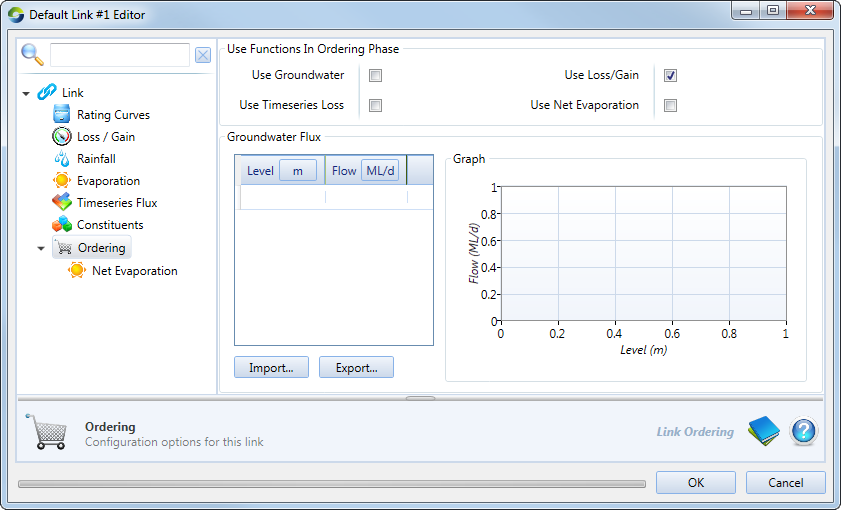
The order coming into the routed link is adjusted to cater for the lateral fluxes over each time-step that the ordered flow spends in the link.
Ordering with ownership
When ownership is enabled in Source, every water order is associated with an owner and is generally supplied using that owner’s water. Where there is insufficient water to supply an owner’s order at any location, and another owner has water surplus to their requirements, the owner with a deficit may borrow water from the owner with surplus to help meet demand (Borrow and Payback Systems, Distribution Systems).
Network Linear Programming
Linear programming techniques assume that the data used is perfect. In particular, when activating these features, you are assuming that the objective function and constraint coefficients are correct, rather than the best estimates available. If this assumption does not hold, the solutions found may be sub-optimal.
Within this chapter, the word "solver" means "the chosen linear programming optimisation algorithm".
Solvers use arc-node networks as their inputs. Source creates arc-node networks automatically for each time-step from the node-link network in the Schematic Editor. There may be differences between the solution found by the solver ("as predicted") and flows as modelled during the flow phase ("as released"). The flow distribution phase resolves these differences by considering the ordering phase as having provided a minimum target to aim for. The optimum flow for each arc is determined by the netLP so that water will flow along the least cost pathway.
About costs
The solvers use a scheme of costs to determine optimal flows. Costs can range from -1.1E13 through to +1.1E13. The larger the cost, the greater the disincentive for water to flow along an arc. Conversely, the smaller the cost, the greater the incentive for water to flow along an arc. For example, in the above list of solver priorities, satisfying evaporative and transmission losses have the lowest cost, and therefore the highest incentive, in any model. The question of relative costs becomes relevant when defining cost functions for storages that are being operated in harmony.
Solver priorities
The highest priority of the solver is to preserve mass balance. The remaining priorities are, in order:
- Satisfy evaporation losses in storages;
- Satisfy transmission losses;
- Satisfy minimum flow requirements;
- Satisfy consumptive demand;
- Minimise spills; and
- Where end-of-season targets are specified for storages, ensure these are met.
Linear programming solvers iterate until the solution falls within specified limits. For Source, these limits are defined in the Convergence Criteria fields. These limits apply, per arc and per storage, within the solver.
Choosing an optimisation algorithm
Source offers two basic linear programming algorithms: RELAX-IV and PPRN. From a modelling perspective, neither algorithm is "better" or "worse" than the other. They simply offer different features:
- RELAX-IV is generally faster than PPRN, particularly when PPRN is being run without side constraints. However, under certain circumstances, both PPRN without side constraints and RELAX-IV may become bogged down in excessive iteration;
- PPRN supports side constraints. RELAX-IV does not. If side constraints are crucial to the correct outcome, or to avoid sub-optimal solutions, or to control excess iteration, RELAX-IV can not be used; and
- PPRN uses real numbers (at the precision of the underlying hardware) whereas RELAX-IV works with integers. Selecting the RELAX-IV algorithm implies integer conversion of the real numbers used internally by Source, during the optimisation process. Conversion implies rounding. Source scales values automatically before sending them to RELAX-IV to minimise loss of precision, and reconverts results returned by the solver to the proper range.
Any other algorithms in the list are experimental and should not be used.
If a model is sensitive to travel time, one of the Travel Time Replicates algorithms should be used.
About side constraints
Side constraints are implemented by translating between requirements set in various nodes and links in the Schematic Editor to the arcs and nodes used by the solver. In other words, you do not need to do anything to configure side constraints. Simply choosing PPRN with side constraints activates the necessary translations. For example, a Loss node creates an arc with high incentive that forces the solver to accept a particular loss.
The use of side constraints can reduce modelling time significantly. In the absence of side constraints, the solver iterates towards an optimal solution. The more iterations required per time-step, the greater the computation effort (CPU cycles = time). Side constraints can reduce the number of iterations required per time-step, sometimes to a single iteration. Each side constraint also guarantees implementation of the condition imposed by the relevant node in the Source schematic model.
Side constraints must be expressible as linear relationships for each time-step. In practice, real world phenomena are poorly modelled by straight lines and usually need curves or piecewise linear functions. Experience suggests that modellers often add numerous small line-segments to piecewise linear editors in an attempt to describe real-world behaviour accurately. The greater the number of small line-segments, the greater the risk that an artifact of the process used to derive the linear relationship for a time-step could generate an infeasible solution. Therefore, modellers should consider whether reasonable accuracy could be obtained from a smaller number of line segments. If not, linear programming solutions may not be appropriate.
Other situations where the use of side constraints are indicated include:
- Head versus outlet capacity relationships for storages, providing that the change in head across a single time-step does not also cause a change in the linear relationship (cross a control point in a piecewise linear function);
- Flow dependencies that cause excess iteration; and
- Circular constraints that prevent the solver from converging on an optimal solution.
Configuring optimisation
To configure optimised ordering, begin by choosing or click Configure Ordering on the Ordering toolbar and choose Network Costs.... This opens the Network costs dialog (Figure 3).
Figure 3. Network costs (summary)
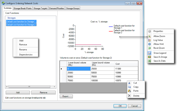
Creating cost functions
By default, Source creates one default cost function for each Storage node in your model. You can add, remove or rename cost functions using a combination of the Add and Remove buttons, and the contextual menu that pops up when you right-click on the list of cost functions. A common pattern is to add cost functions that are applicable to various periods throughout the year. The finest level of granularity supported by Source is a cost function applicable to a single month.
The graph on the right hand side of Figure 3 provides a graphical representation of the selected storage cost. You can also simultaneously display several functions based on your selection of storage cost functions from the list on the left hand side. The lower the cost (Y-axis) the greater the incentive to retain, or carry-over the associated storage volume (X-axis) to the next time-step. The same information is presented in the table, and can be exported to a .CSV file if required.
You can rename cost functions or display dependencies using the right-click contextual menu. A dependency is the association between a cost function and a storage. This can be useful if the name you choose for a cost function does not include the name of the storage for which it was defined.
Designing cost functions
Use the Storage Break Points tab (Figure 4) to design cost functions. Begin by using the Storage Cost Function pop-up menu to select a cost function that you defined in the Cost Functions list in the Summary tab. Next, select the storage that should be associated with this cost function.
Figure 4. Network Costs (Storage Break Points)

By default, Source provides four rows in the Break points table. Each row is associated with a percentage of the full supply storage volume, which is visible, and a cost, which is not visible. In the Break points table shown in Figure 4:
- The bottom-most 10% of the capacity of the storage is associated with a base cost of -11000.00;
- The next 40% (50%-10%) of the capacity of the storage has a cost of the base cost plus one unit of increment. Here, the increment is 10, so the cost will be -10990;
- The next 30% (80%-50%) of the capacity of the storage has a cost of -10980 (base plus two increments); and
- The remaining capacity of the storage has a cost of the base plus three increments: -10970.
A more formal specification of the cost calculation is:

Recall that negative costs are incentives. Accordingly, in this table, the greatest incentive is to retain any water in the bottom-most 10% of the capacity of the storage (for carry-over to the next time-step), followed by the water in the next 40% of the capacity of the storage. By interleaving base costs and increment values, releases from multiple storages can be controlled quite precisely to maintain a desired balance.
Although Source provides four rows by default in a Break points table, you can define as many, or as few breakpoints as you need. The rules are:
- There must be at least one breakpoint and the first breakpoint must be numbered 1;
- Breakpoint numbers must increase monotonically down the table. If you edit a number so that it is more than one higher than the previous number, then close and re-open this dialog, Source will automatically insert the missing numbers and distribute the storage percentage capacity across them;
- Storage percentage numbers must increase monotonically down the table. The storage percentage associated with the first breakpoint may be zero; and
- The storage percentage in the final row must be 100%.
As you edit the breakpoint table, Source constantly checks that these conditions hold and places alert symbols next to offending values. Because of this, it may be necessary to visit each cell containing an alert symbol to force the integrity check. Alternatively, it may be easier to import more complex breakpoint tables from a .CSV file. The format of the file is shown in Table 1.
Table 1. Storage breakpoints (data file format)
| Row | Column (comma-separated) | |
|---|---|---|
| 1 | 2 | |
| 1 | Carry over number | Active storage (%) |
| 2..n | n | point |
where:
n is an integer in the range 1..n representing the carry-over number
point is the storage percentage (eg. “10” for 10%) when carry-over arc n takes effect.
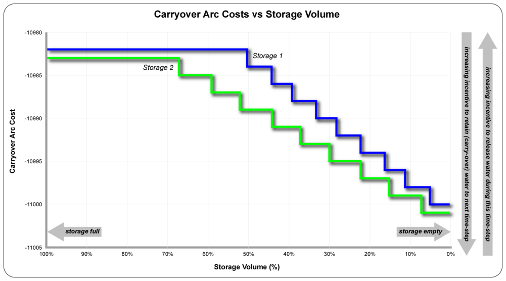
To understand how cost functions work, consider Table 2 which shows the definition of cost functions for two storages that are intended to operate in parallel. The design intention is:
- Storage 1: the first 50% of this storage should be used first, after which its remaining capacity should be consumed in 9 equal steps of 5.6% each (50%÷9=5.6%);
- Storage 2: When storage 1 reaches 50% of its capacity, 33.3% of the capacity of storage 2 should be used, after which its remaining capacity should be consumed in 9 equal steps of 7.4% (66.6%÷9=7.4%); and
- Once the initial consumption levels have been achieved (ie. 50% of Storage 1, 33.3% of Storage 2), the two storages will be drawn down in proportion to each other.
Table 2. Storage cost functions (example)
| Storage Carryover Arc | Storage 1 | Storage 2 | ||
|---|---|---|---|---|
| Base Cost | -11000 | Base Cost | -11001 | |
| Increment | 2 | Increment | 2 | |
| Storage % | Arc Cost | Storage % | Arc Cost | |
| 1 | 5.6 | -11000 | 7.4 | –11001 |
| 2 | 11.1 | -10998 | 14.8 | –10999 |
| 3 | 16.7 | –10996 | 22.2 | –10997 |
| 4 | 22.2 | –10994 | 29.6 | –10995 |
| 5 | 27.8 | –10992 | 37.0 | –10993 |
| 6 | 33.3 | –10990 | 44.4 | –10991 |
| 7 | 38.9 | –10988 | 51.9 | –10989 |
| 8 | 44.4 | –10986 | 59.3 | –10987 |
| 9 | 50.0 | –10984 | 66.7 | –10985 |
| 10 | 100.0 | –10982 | 100.0 | –10983 |
The result of the design intention is shown in Figure 5. Note that, in the absence of any inflows that replenish the storages, the X-axis can also be interpreted as expressing time.
Figure 5. Carryover Arc Costs vs Storage Volume
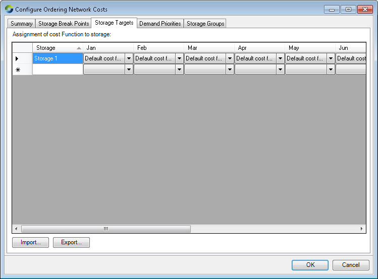
Applying cost functions
You apply cost functions in the Storage Targets tab (Figure 6). Each storage in your model is represented by a row in this table. The remaining columns contain pop-up menus where you can connect an appropriate cost function to a selected storage for a particular month.
Figure 6. Network costs (Storage targets)
You can also import storage targets from a .CSV file. The format of the file is shown in Table 3. Note that the column ordering in the .CSV file does not match the display in Figure 6.
Table 3. Storage targets (data file format)
| Row | Column (comma-separated) | |
|---|---|---|
| 1 | 2..13 | |
| 1 | Storage | month |
| 2..n | sname | cname |
Where
month is the first three characters of the month of the year (eg “Feb”)
sname is the name of the storage
cname is the name of the storage cost function.
Controlling shortfall
A shortfall occurs when insufficient water is released to meet a demand. The arc-node model built by Source deals with this contingency by providing alternative, high-cost paths of last resort. These paths are known as shortfall arcs and their presence allows the model to satisfy mass balance.
You can specify the number of shortfall arcs that are generated for each of the demand nodes using the Number of Shortfall Arcs drop down menu (Figure 7). The default number is 4.
Figure 7. Network Costs (Demand Priorities)
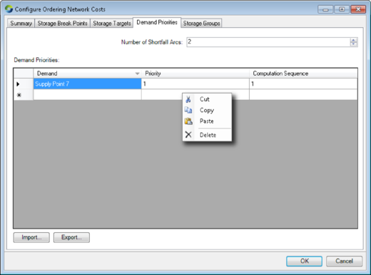
You can control the order in which shortfalls are satisfied. The Priority column in Figure 7 shows which demand component of the model has will receive water via its shortfall arcs.
You can import shortfall demand priority rules from a .CSV file. The format of the file is shown in Table 4.
Table 4. Demand priorities (data file format)
| Row | Column (comma-separated) | ||
|---|---|---|---|
| 1 | 2 | 3 | |
| 1 | Demand | Priority | Computation Sequence |
| 2..n | sname | pri | seq |
Where:
sname is the name of the supply point
pri is the priority number
seq is the sequence number
Table 5 shows the result of adjusting the priorities and computation sequences of a scenario containing two demand nodes. When priorities are equal, the first arc of the demand node with the highest computation sequence number is satisfied first, then the first arc of the demand node with the second-highest computation sequence is satisfied, and so on in round-robin fashion until either all arcs are filled or no more water remains. When priorities are unequal, all arcs of the demand node with the highest priority number are satisfied first, then the allocation moves to the demand node with the next-highest priority number, and so on until either all arcs are filled or no more water remains. You can combine priorities and computation sequences to achieve any desired outcome.
Table 5. Shortfall arc costs (example)
| Scenario | Supply point | Priority | Computation sequence | Shortfall arc | Satisfaction order | |
|---|---|---|---|---|---|---|
| Number | Cost | |||||
| A | 1 | 1 | 1 | 1 | 11000002 | 2 |
| 2 | 11000004 | 4 | ||||
| 3 | 11000006 | 6 | ||||
| 4 | 11000008 | 8 | ||||
| 2 | 1 | 2 | 1 | 11000001 | 1 | |
| 2 | 11000003 | 3 | ||||
| 3 | 11000005 | 5 | ||||
| 4 | 11000007 | 7 | ||||
| B | 1 | 1 | 2 | 1 | 11000001 | 1 |
| 2 | 11000003 | 3 | ||||
| 3 | 11000005 | 5 | ||||
| 4 | 11000007 | 7 | ||||
| 2 | 1 | 1 | 1 | 11000002 | 2 | |
| 2 | 11000004 | 4 | ||||
| 3 | 11000006 | 6 | ||||
| 4 | 11000008 | 8 | ||||
| C | 1 | 2 | 1 | 1 | 11000001 | 1 |
| 2 | 11000002 | 2 | ||||
| 3 | 11000003 | 3 | ||||
| 4 | 11000004 | 4 | ||||
| 2 | 1 | 1 | 1 | 11000005 | 5 | |
| 2 | 11000006 | 6 | ||||
| 3 | 11000007 | 7 | ||||
| 4 | 11000008 | 8 | ||||
NetLP ordering at nodes
In Source, networks are composed of arcs which have maximum capacities and costs associated with them. These costs can either be positive (disincentive) or negative (incentive). The optimum flow for each arc is determined by the netLP so that water will flow along the least cost pathway.
While the minimum and maximum order times have to be calculated upstream of each relevant node to the relevant storages, the system also has to calculate the downstream order time which is the timeframe over which the node must forecast the downstream orders for in advance.
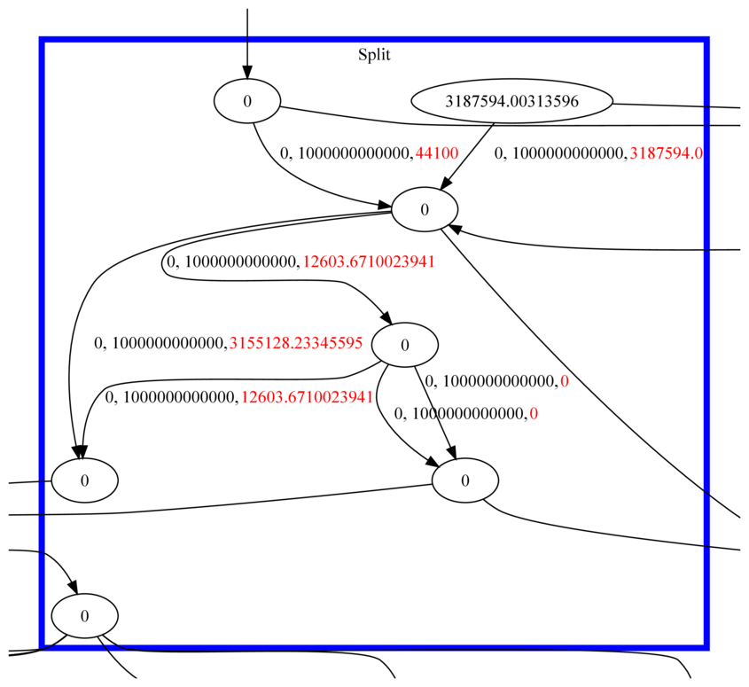
For the splitter node, in the netLP order phase, the main stream has two parallel arcs - a forced flow arc and the natural flow arc. The capacity of the forced flow arc in the mainstream is the opposing flow volume of the maximum effluent flow. The maximum effluent flow is dependant on the inflow to the controlled splitter node. The effluent side of the controlled splitter also has a forced and a natural flow arc, with the capacity of the forced flow arc the minimum volume of flow down the effluent side.
Rules for the flow phase handling of orders are:
- If the flow phase inflow of the node is higher than the order phase, then all excess flow will be sent down the main stream; and
- If the flow phase inflow of the node is lower than the order phase, then each side of the splitter will be apportioned water according to the proportion of the order phase main stream and effluent flows to the order phase splitter inflow.
To ensure that the above are met, you can configure each of the branches with a cost incentive. In a maximum flow constraint node that is immediately below the controlled splitter on one side of the stream, this will ensure that the flow rules are met. The maximum flow constraint should be configured with parallel arcs with either a cost for flowing water down the effluent or a cost incentive for flowing water down the main stream. The cost should be small, to ensure that the overall cost structure of the network is not impacted too much. Figure 12 shows an example of this.
Inspecting an arc-node network (simple)
It is possible to inspect textual representations of the arc-node networks that are generated by Source for processing by the solver. The steps are:
- Select the active scenario in the Project Hierarchy (Project Explorer);
- Locate the Arc-Node Network entry in the Model Parameters list (also Project Explorer) and enable it for recording;
- Run the scenario; and
- In the Values column of the Recording Manager (Complex time series, summary), locate and open View Multiple Supply Path Setup. The window will be similar to Figure 9.
Figure 9 is a work in process so most of the labels are inaccurate. The graph provides a measure of computational complexity (iterations to solve) at each time-step. Note that the peaks are clipped to the value of the Maximum Iterations parameter in Figure 1.
Figure 9. Inspecting the generated arc-node model
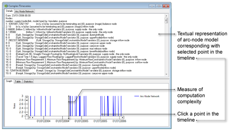
Clicking any point in the time line causes a textual representation of the arc-node model for that time-step to be displayed in the upper part of the window. The text can be selected and placed on the clipboard for re-use.
Note that it is beyond the scope of this guide to explain the format of the arc-node model dump.
Inspecting an arc-node network (advanced)
It is also possible to visualise the arc-node networks that are generated by Source. However, you will first need to download and install a third-party software package called Graphviz. The home page for this application is:
Choose the current stable release in preference to any development snapshots. Consult your Windows system administrator if you need help installing Graphviz.
To enable debugging and visualisation support in Source:
- Choose (Figure 1);
- Enable Export iterations;
- If your model operates over a large number of time-steps, you may wish to restrict the date-range for which arc-node output is produced using the Start and End date controls in Figure 1; and
- Click OK.
Next, run your model. Enabling Export iterations creates a folder on your Desktop with a name in the pattern:
MspNetworkOutput-yyyy-mm-dd
At the end of a run, this folder will contain three files per time-step:
- A visual representation (.DOT) of the arc-node network suitable for display in Graphviz;
- A textual representation of the arc-node network; and
- A textual representation of the test case for that time-step.
To visualise an arc-node network for a given time-step:
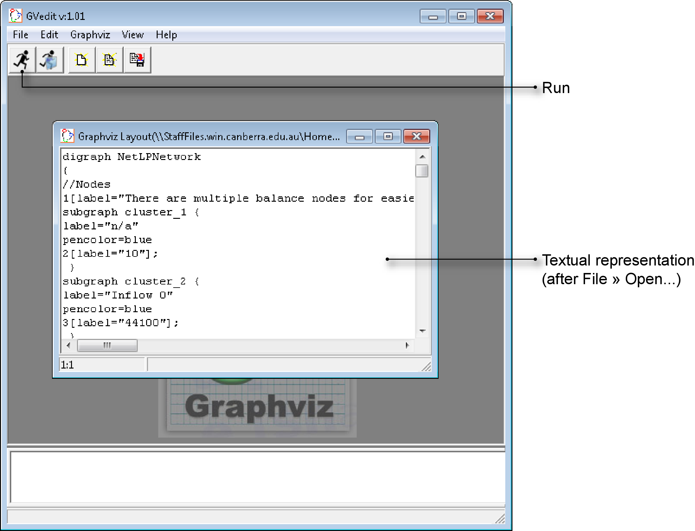
- Use the Windows Start menu to launch Gvedit, which is part of Graphviz;
- Choose and select the .DOT file of interest. Gvedit will respond by opening a textual representation of the arc-node network as shown in the central window in Figure 10; and
- Click the Run button on the Gvedit toolbar (Figure 10).
Figure 10. Gvedit (opening an arc-node network)
Graphviz always generates a graphical representation of your arc-node network in two forms. One is displayed on your screen and the other is saved as a file. By default, the version saved as a file is in .GIF format but you can change this using the Output File Type pop-up menu in Figure 11. Note that Graphviz can also generate high-resolution vector-based representations such as .SVG.
By default, the file is saved in the same folder as the original .DOT file. You can change this by clicking the ellipsis button (...) to the right of the Output File Name field in Figure 11.
Figure 11. Graphviz settings dialog
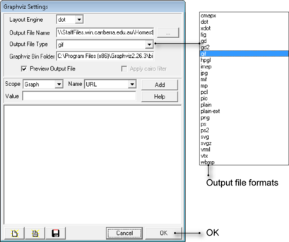
Once the settings have been configured to your requirements, click OK. Figure 12 is an excerpt from an arc-node network diagram produced by Graphviz. The elements inside the blue rectangle correspond with a Splitter node in the original Source schematic.
Figure 12. NetLP arc-node network for Splitter node