Running scenarios
Introduction
A Source scenario must be run in order to produce any useful information. Each scenario run produces a collection of result sets. A result set is a group of related outputs, usually from the same component and is usually, but not always, arranged as a time series.
During a run, each component in the scenario can produce one or more result sets in the form of predicted water flows, volumes and other outputs specific to that component. Some components are capable of producing more than 20 separate result sets. When ownership is not enabled, the model starts at the first node then progresses down the river system in a single pass to compute the water volume and flow rates through each node and link.
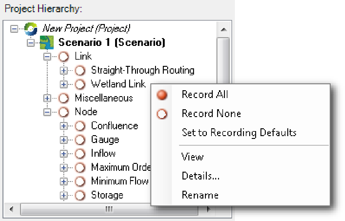
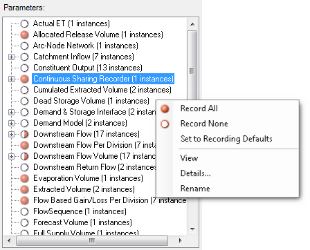
Figure 1. Selecting recording parameters
Running a scenario
To run a scenario, do the following:
- Select the model outputs of interest. Some model outputs are selected by default; you can change which outputs are recorded by default;
- Click Select Analysis Type on the Simulation toolbar to set the appropriate type of analysis. Depending on the scenario, Source offers several options for analysing your model data, including:
- Flow calibration analysis, which calibrates a set of rainfall-runoff and flow routing model parameter values so that output from the model is representative of an observed data set;
- Run w/Warm Up, which seeds the model with the available historical data and prepares for forecasting. This is enabled in River Operations scenarios only;
- Single analysis, which simulates the river performance for a single set of conditions (as opposed to an iterative analysis which considers several possible outcomes); or
- Stochastic analysis, which is used to generate flow replicates from stochastically generated rainfall inputs when dealing with stochastic climate data. See also Incorporating uncertainty into climate variability.
- Click Configure on the Simulation toolbar to select the required time frame for the scenario to run. The resulting window depends on the type of analysis you chose in the previous step. If you chose:
- Flow Calibration analysis, the Calibration Wizard opens. Refer to Calibration Wizard for catchments;
- Run w/Warm Up, the Run w/Warm Up window opens (Run w/Warm up);
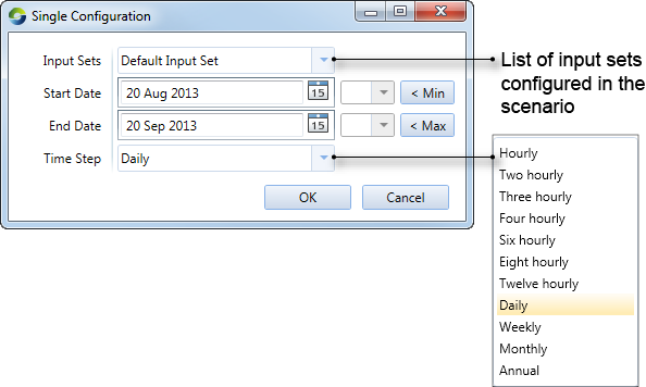
- Single analysis, the Single Analysis window opens (Figure 2); or
- Stochastic analysis, the Stochastic Analysis Tool opens. Refer to Using the stochastic analysis tool.
You can only configure a run time frame that is supported by the time spans in the time series associated with your scenario. A lowest-common-denominator approach is used. For example, if your project contains two time series where the first spans the period 1/1/1900 through 31/12/1990, and the other the period 1/1/1960 through 21/12/2010, the available simulation time frame will be 1/1/1960 through 31/12/1990.
- Click Begin Analysis (Run) on the Simulation toolbar to start the simulation run.
Figure 2. Configure single analysis
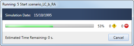
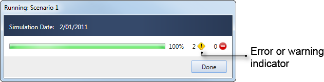
While the scenario is running, you will see a progress bar (Figure 3) displaying the percentage of the scenario completed, estimated time to completion and the current time-step being processed.
Figure 3. Running scenario (progress bar)
Component-level controls
Whether any given result set is produced by any given run of a scenario is controlled by whether the result set’s recording parameter is enabled or disabled for that run. To adjust the state of recording parameters for a component, first select the component within the Project Hierarchy. Then do one of the following:
- To record all the available parameters for a component, right-click on the component and choose Record All from the contextual menu (Figure 1);
- To disable the recording of any parameters for a component, right-click on the component and choose Record None from the contextual menu (Figure 1); or
- To restore the model parameters for a component to their default value, right-click on the component and choose Set to Recording Defaults from the contextual menu (Figure 1).
Parameter-level controls
For fine-grained control of individual recordable parameters:
- Select the component within the Project Hierarchy. Selection causes all of the component’s parameters to be displayed in the Model Parameters area (Figure 4); and
- Use the contextual menu (right-click) to selectively enable or disable individual parameters or parameter groups, or to restore parameters to their default settings (Figure 4).
Figure 4. Selecting model parameters
Scope of contextual menus
The contextual menus shown in Figure 1 and Figure 4 can be applied at any point within their respective hierarchical displays. If you select an individual component or parameter, the effect will be limited to just that element. Applying a recording choice at an aggregate level propagates the effect to the selected element and all elements below it in the hierarchy.
Setting recording defaults
Choosing Recording Defaults... from the View Type pop-up menu on the Project Explorer toolbar opens a window where you can specify the parameters which should be recorded by default for each kind of component. See also Recording Manager defaults. Changes made in this window persist across invocations of Source.
Recording model outputs
When you run the models in a scenario, every node and link produces results in the form of predicted water flows, volumes and other data outputs.
Some node or link types can produce more than 20 separate data outputs (eg. storages). In general, the more outputs you record, the longer the simulation will take, though this depends on exactly what you record; recording mass-balance is more computationally intensive than recording inflow, for example.
When you save a project, or make a copy of a scenario, Source automatically saves the list of model outputs selected for recording. There are two ways to select which parameters and model elements to record:
- Using the Project Explorer, right-click a node, link or other element in the Project Hierarchy or a model parameter (Figure 4). From the pop-up menu, select:
 Record all: every parameter at this level and below will be recorded;
 Record none: no parameters at this level and below will be recorded;
If the indicator appears as , this shows that some (not all) parameters at this level and below will be recorded.
- If you select a model element on the Geographic Editor or Schematic Editor (eg a catchment outlet), then the chosen model element is highlighted in the Project Hierarchy. Right-click the element name and select the recording status from the pop-up menu, or click the Record icon in the Project Explorer toolbar.
Using the Log Reporter
If a scenario run results in errors or warnings, the first indication of those is displayed in the Run completion dialog by a red or yellow icon next to the Close button as indicated in Figure 5.
Figure 5. Running scenario (error)
You can investigate the causes of errors or warnings using the Log reporter (Figure 6). If the Log Reporter window is not visible, do either or both of the following:
- Choose to make it visible; and
- Make the Log Reporter active by clicking the Log Reporter tab.
Once the Log Reporter is active, you can view all the logs run by Source, from configuring a scenario to running it. To clear the log, right-click the Log Reporter window and choose Clear from the contextual menu. To copy log contents to a .csv file, right-click the Log Reporter window and choose Export from the contextual menu. Table 1 shows what each of the columns stand for.
Figure 6. Log Reporter
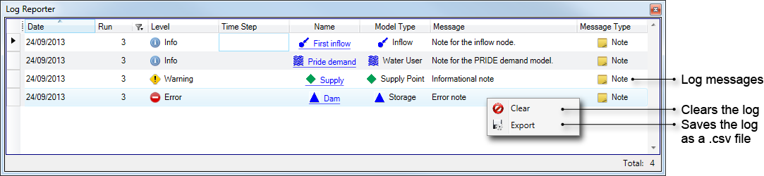
Table 1. Log Reporter, Columns
| Column | Description |
|---|---|
| Date | The local date on the computer. |
| Run | The run number. You can also filter messages based on this number - use the filtering icon. |
| Level | The type of message (similar to notes) - informational, warning or error. |
| Time Step | The scenario time-step which the message refers to. |
| Name | Name of the node or link corresponding to the message. |
| Model Type | These are the node and link types – ie. Inflow, Straight Through Routing |
| Message | Details of the message. |
| Message Type | There are three types available:
|
Scenario results
Each scenario run creates a distinct collection of result sets. Each collection is represented by a tab in the Recording Manager. The name of each tab is formed by concatenating the name of the scenario with a time-stamp indicating when the scenario was run. For example, Figure 7 shows that "Scenario 1" has been run twice at slightly different times.
Figure 7. Recording Manager
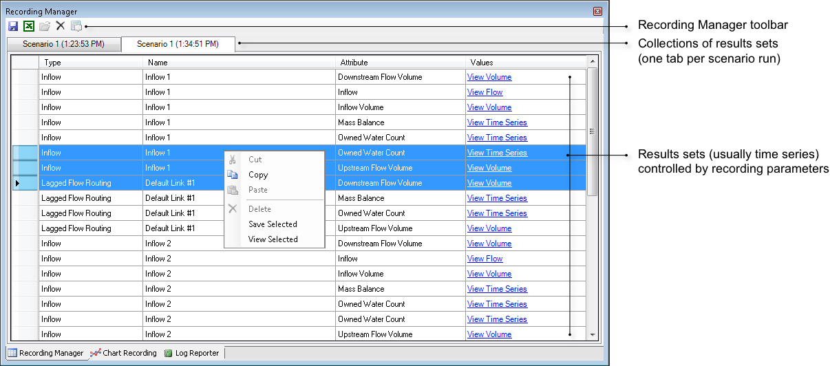
You can use the tools on the Recording Manager toolbar to save a collection of results to a file, export a collection to Microsoft Excel, or delete the currently-selected collection.
Within each of the Recording Manager’s tabs, results are arranged in four columns:
- Type - Source generic name for node or link (eg Inflow);
- Name - your name for that component;
- Attribute - the name of the output parameter as listed in Parameters (eg Additional Inflow); and
- Values - a link which can be clicked to view a graphical representation of the output parameter.
You can navigate through a list of results using the vertical scroll bar. In addition, clicking on a link or node in the Schematic Editor, Geographic Editor or Project Hierarchy automatically selects all of the result sets associated with that component in the Recording Manager.
Right clicking in the Recording Manager, then choosing Save Selected allows you to export the selected time series data as a .csv file. Choosing View Selected opens the Charting Tool for the selected time series data.
One of the key uses of the Recording Manager is to select one or more result sets (rows in the Recording Manager) for display in the Charting Tool. The Charting Tool helps you visualise, analyse and understand scenario results and other data produced by Source. Each time you click a link in the Values column, a copy of the Charting Tool opens to display that result set. Clicking the same link multiple times opens additional copies of the Charting Tool containing the same result set.
You can also use the Chart Recording Manager to view and manage result sets. Refer to Chart Recording Manager for more information.
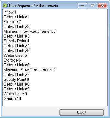
Determining the flow sequence
You can find out how flow travels through the model by enabling the Flow Sequence model parameter prior to running the model. Click on Miscellaneous in the Project Hierarchy, which will populate the Parameters list with various attributes. Right click on Flow Sequence and choose Record All from the contextual menu. This attribute can be viewed in the Recording Manager and lists the nodes and links which describe the flow sequence (from the Flow Distribution Phase) in the model run. You can export this list using the Export button as shown in Figure 8.
Figure 8. Recording manager, Flow sequence
Using the Tabular Editor
The Tabular Editor only contains information after a warm-up or scenario run and is positioned to the first time-step in the forecast period. Figure 13 has been adjusted slightly to show both historical and forecast data. The row where the cells have a pale blue background is the first day of the forecast period (ie. normally “today”). Rows prior to this show historical data. At this point, all values in the forecast period are zero because no forecasting has been done.
Figure 13. Tabular Editor
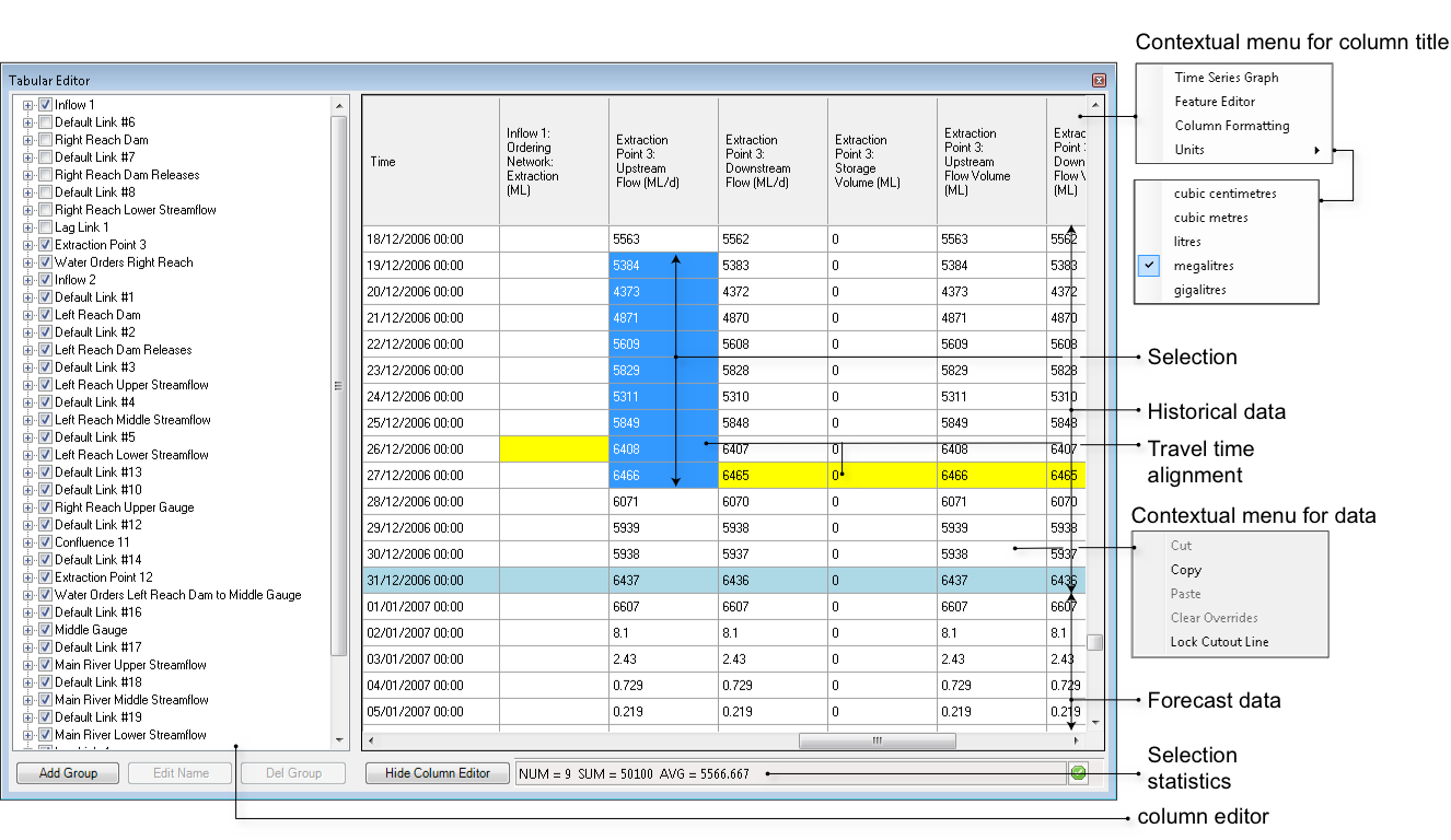
Clicking the column title opens the Charting Tool for the node’s time series. This is synonymous to right clicking and choosing Time Series Graph from the contextual menu (Figure 13). Choosing Feature Editor opens the node’s feature editor that is associated with that column. Additionally, the contextual menu provides a means of changing the column’s units and access to a formatting editor for the individual column (see Customising the Tabular Editor).
Clicking a cell shows the relationship between nodes corrected for travel time. Figure 13 shows this relationship using a yellow highlight. When multiple cells are selected:
- The travel-time indicator is only calculated for the last cell that was clicked; and
- The selection statistics are updated to show the sum and mean for all cells in the selection.
The Show Column Editor button expands the window (Figure 13) to include an hierarchical list of data sources that are candidates for inclusion in the Tabular Editor. Click Hide Column Editor to return to the original view.
Using the Column Editor
The Show Column Editor tab displays a tree view of all the nodes used in the scenario, which you can expand to show the output parameters for each node. You can change the way results are displayed in the Tabular Editor, making analysis easier. You can:
- Check or uncheck items in the list to show or hide the relevant columns in the table.
- Re-order columns by clicking and dragging an item to the desired location in the list. For example, Figure 14 shows how re-ordering the parameters in the list results in a re-arrangement of table columns. In this case, the Downstream Flow for Storage 2 and Storage 4 appear together in the table after re-ordering them in the column editor.
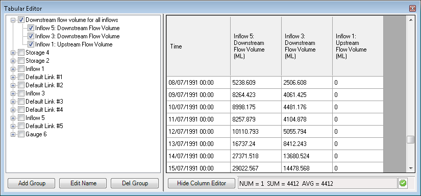
Group similar parameters together using the group-related tabs. Click on Add Group and enter an appropriate name for the group. Add the desired parameters, nodes or links by clicking and dragging them into the new group. An additional group (Downstream flow volume for all inflows) has been added to the list in Figure 15, along with the relevant parameters from each inflow node. This group can be renamed (Edit Name) or removed (Del Group).
Figure 14. Show Column Editor (Column re-ordered)
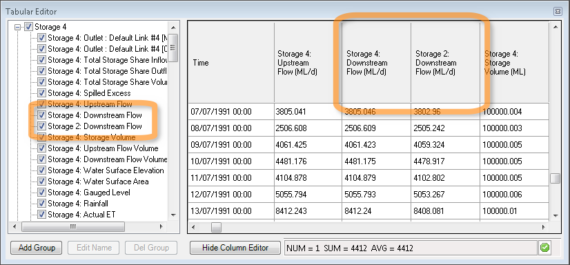
Figure 15. Show Column Editor (Add group)
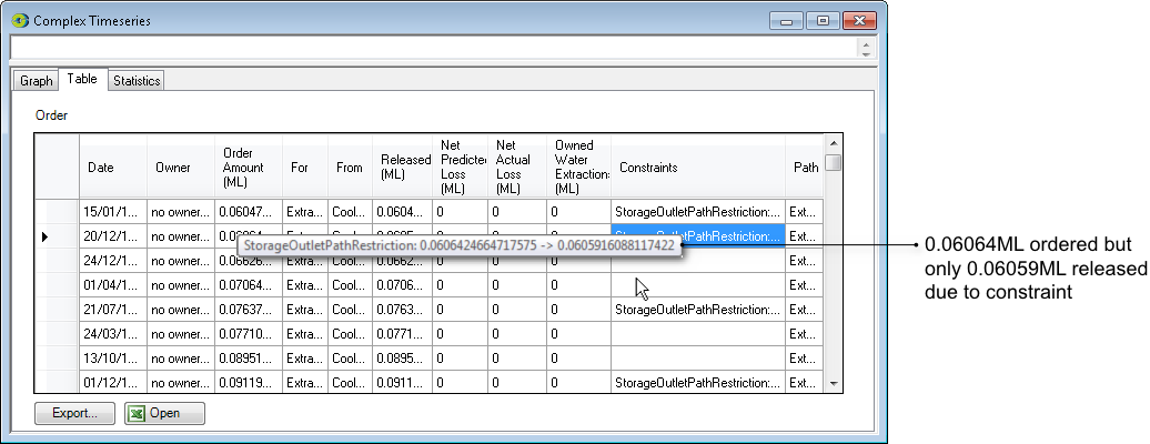
Identifying constraints
When constraints are enforced, there may be a difference between the amount of water ordered and that released. The application of constraints is evident at both the supply point and minimum flow requirement nodes.
To discover where constraints have been applied:
- Run the model;
- Select an appropriate supply point or minimum flow requirement node. This selects all of the node’s recording parameters in the Recording Manager; and
- Inspect the Values column in the Recording Manager and click an Order Details link. This opens a Complex Time Series Form (Figure 16). The Graph tab provides a summary of the differences between the amount ordered and the amount released for the duration of the run. The Constraints column of the Table tab (Figure 17) provides a breakdown per time-step. Hover your mouse cursor over a cell of interest to see its contents presented in a tool-tip.
Figure 16. Complex time series (Orders vs Releases, summary)
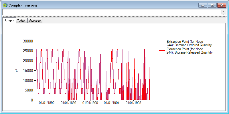
Figure 17. Complex time series (Orders vs Releases, detail)