Forecasting
Introduction
Operations forecasting allows you to create alternate forecasts for inflows, water demands, stream flow losses and gains (unaccounted differences) and constituents within a single overall project scenario. In other words, it forecasts the input data for a model. This is not available in Source (public version).
The Operations simulation in Source is split into two phases - the historic 'warm-up' and the forecast period. The former is designed to warm-up the network's physical models by playing all known historic data into the system and overriding modelled values where applicable. In the latter, the Operations forecast models extend historic data into the future, effectively providing an estimate of the effect to the modelled system.
To create a default operations scenario in Source:
- First, create a manager scenario;
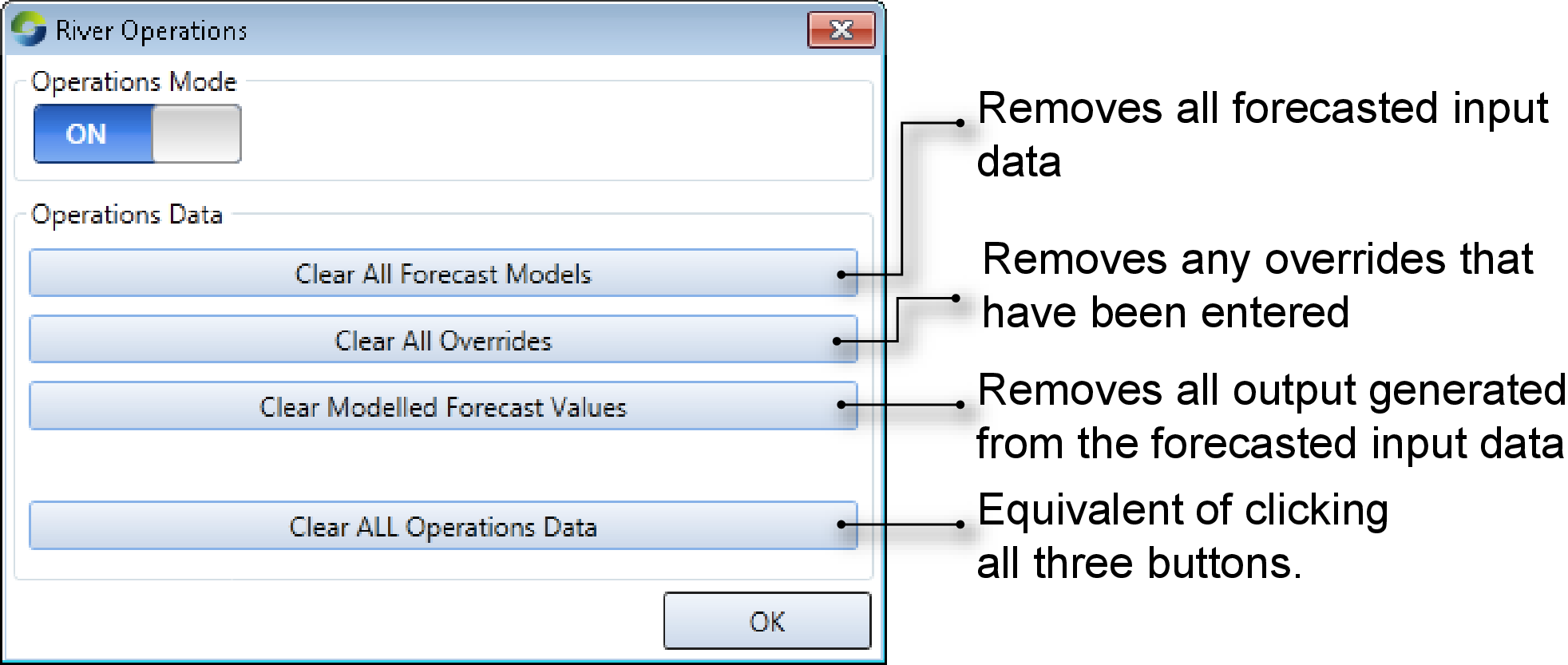
- Choose Tools » River Operations to open the River Operations dialog (Figure 1); and
- Click on the slider below Operations Mode to ON.
Once you have created forecast models, you can disable operations, but retain these models or overrides using the buttons under Operations Data. The first two buttons in this dialog deal with removing input data, whereas the third one deletes all output data that was created for the forecast models. To clear all operations related data (input, output as a well as overrides), click Clear ALL Operations Data.
Figure 1. River Operations
Warming-up the model
Before you can begin forecasting, you must seed the model with available historical data (also known as "warming-up the model") using the Simulation toolbar:
- Choose Run w/Warm Up from the Select Analysis Type pop-up menu; and
- Click Configure.
This opens the Run w/Warm Up dialog (Figure 2).
Figure 2. Run w/Warm Up
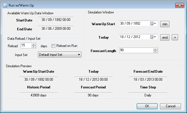
Assuming a daily time-step:
- The Start Date and End Date fields define the limits of the available historical data in your model;
- The Warm Up Start date is set to the beginning of your historical data but you can change this if you intend to limit the warm-up process to a shorter time span;
- The date for Today is set to the last day of your historical data but you can also adjust this field as appropriate. Assuming your historical data is up-to-date (yesterday was the last day of historical data), this value should normally be today’s date so any difference might indicate a need to verify that all data has been loaded correctly into the model; and
- The Forecast Length defaults to 90 days. You would usually set this to the maximum travel time associated with your normal operations.
The + button can be used to step the operations scenario forward in time, which allows you to move from one day’s operational scenario to the next. You can also specify the data source using the Input Set drop down menu.
The remaining fields summarise what will occur when you complete the warm-up process. Click OK, and then Begin Analysis (Run) to begin the warm-up process.
Creating forecasts at nodes
Once operations has been enabled, you can configure forecast input data under the relevant forecasting list item in a node's feature editor. For example, for the inflow node, choose Inflow Forecast under Additional Flow. Each of the parameters that are involved in creating forecasts handle input data differently.
The following forecast models extend the originally played in time series using a model. In the absence of a forecast model to generate forecast values, a default value is used, which is typically zero:
- Additional flow at the Inflow node;
- Demand at the Time Series demand model;
- Operating target, gauged releases, rainfall and evaporation for the Storage node.
The Unaccounted difference node and the Gauged Level unaccounted difference at the storage node forecast unaccounted difference forecast the possible error. The default value in the absence of a forecast model is zero. The Unaccounted Difference is a time series computed during the historic phase of the run, and is the difference between the modelled value at a point in the system and the actual historic value which has been played in at that point. In the forecast phase, applying the forecast unaccounted difference (a positive value represents a gain; a negative value, a loss) is an attempt to compensate for the known over or under estimation inherent in the model.
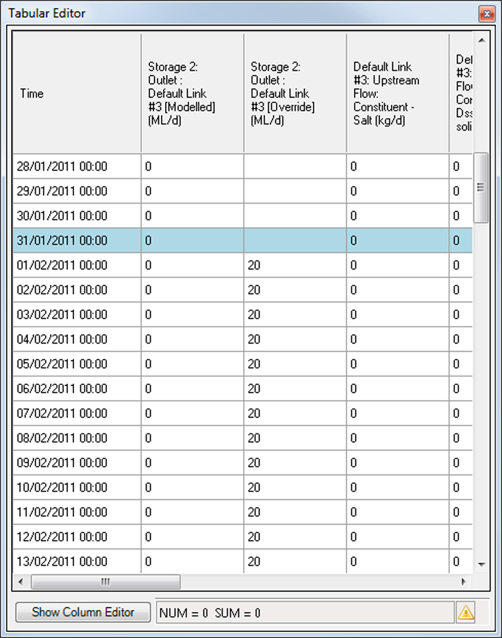
For gauged releases forecast at the storage node, by default, the modelled releases are used by outlets, except where an override value has been provided, either by direct override (using the tabular editor) or by a forecast model. A storage outlet is a physical structure which has minimum and maximum release capabilities. The outlet release forecast/override can be any value, but the model cannot physically release any amount. The forecast/override values are therefore constrained at run-time. This is why the outlet releases each have two columns in the tabular editor, the first shows the modelled value that is actually released by the storage and the second shows the forecast/override. They will be different if the outlet release has been constrained. The second column is blank in the absence of any forecast/override values and in this case, the modelled values are used. Figure 3 shows an example of this. Note that from the 01/02/2011 onwards, the outlet release has been constrained.
Figure 3. Tabular Editor, forecasting, outlet release constrained
Forecast scenarios
A collection of one or more forecasting models is known as a forecast scenario. You can define one or more scenarios for each node. For example, you might define "wet year", "dry year" and "normal year" scenarios, or variations that reflect your most optimistic or pessimistic expectations. To add a forecast scenario, right-click on the item you want to forecast in the relevant node's feature editor and choose Add Forecast Scenario (Figure 4). You can choose the input set that will be associated with a particular forecast scenario. Right click on Forecast Scenario #<number>, then choose Add Forecast Model to add a model.
When more than one forecast model has been assigned to a forecast scenario, they are ordered from top to bottom in the hierarchical list. The model at the top of the list runs first. You can change the order of model run by dragging the forecast model to the required position in the list. For each model, you must also specify the number of time-steps it will be active for before moving onto the next model in the list. The last model in the list always has a Time Steps value of All Remaining and will be active for the remainder of the forecast period.
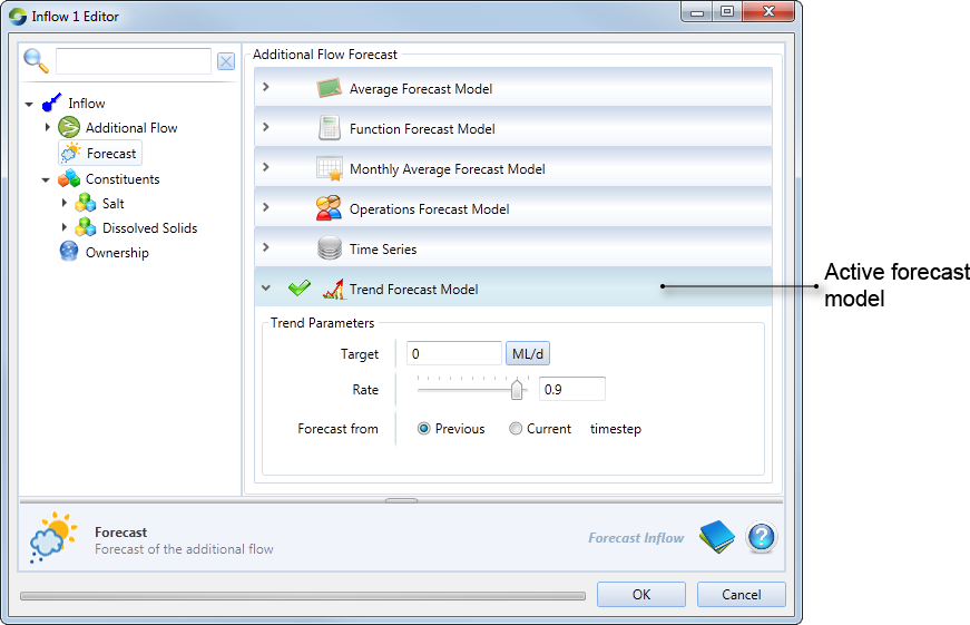
Figure 4 shows the Forecast item for the Inflow node. Choose the forecast model you wish to specify by clicking the appropriate forecast model under Additional Flow Forecast (on the right). The forecast model that is active at the node is indicated by a green tick on the left of the model. In Figure 4, the Trend forecast model is the active model.
Figure 4. Inflow node, Operations forecasting
Forecasting models
Source supports the forecasting model types shown in Table 1.
Table 1. Forecast model types
Forecast model type | Description |
|---|---|
| Average | Average over the last specified time-steps |
Function | User defined arithmetic expressions/functions |
Monthly Average | Daily average for the month in megalitres per day. |
Time Series | Supports the inclusion of forecast data using data sources. |
Trend | A single target value (either positive or negative) plus a recession rate. |
Average forecast model
This allows you to define the average over the last specified number of time-steps.
Function forecast model
You can define an expression or function to return any value you choose for each time-step in the forecast period. For example:
- a fixed value; or
- a fixed proportion of a variable that is available to the Function Editor.
Monthly Average forecast model
Creating a monthly average forecast model allows you to enter an average forecast value, in megalitres per day, to be applied for the whole of each month. You can either enter the monthly average values manually, or import the values from a .CSV file formatted as shown in Table 2.
To trend from "today" to the monthly average, enable the Trend to Value at Rate checkbox and enter a trend rate which is a real number greater than zero but less than one. The observed daily flow rate for the previous month and the number of days of the current month are used to determine the initial flow volume.
Table 2. Monthly average forecasting model (data file format)
| Row | Column (comma-separated) | |
|---|---|---|
| 1 | 2 | |
| 1 | Month | Forecast Value (ML/d) |
| 2..n | month | value |
Time Series forecast model
To specify a forecast based on a time series, you must:
- use data sources to load a time series or scenario; and
- specify the number of time-steps that the model will run in.
Time series are assumed to conform with the structure shown in Table 3. Note that any time-stamps contained in a time series are ignored. The observation in the first row of the time series is used for the first time-step of the forecast period, the observation in the second row for the second time-step, and so on, until either there are no more data rows in the time series or the simulation reaches the end of the forecast period.
Table 3. Time series forecasting model (data file format)
| Row | Column (comma-separated) | |
|---|---|---|
| 1 | 2 | |
| 1..n | date | value |
Trend forecast model
To specify a trend forecast, enter the target value in megalitres per day, and use the slider to specify the trend rate, which is a real number greater than zero but less than one.
Viewing forecasts
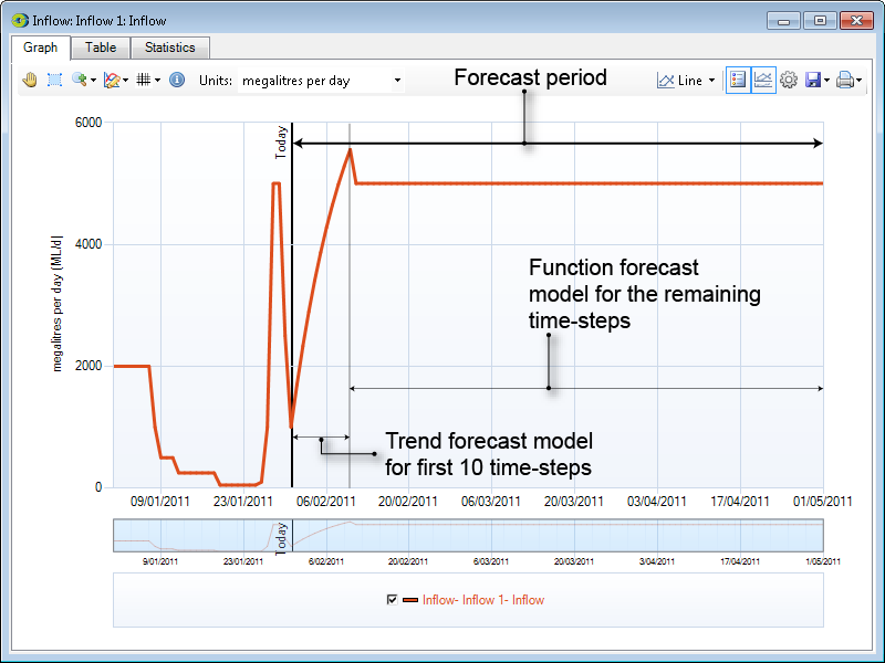
The results of executing one or more forecast scenarios can be viewed using the Recording Manager or the tabular editor (to view and override individual values). Ensure that you enabled recording for the parameter that you are forecasting. For example, to forecast flow, enable recording of the Inflow attribute in the Recording Manager. Figure 5 shows an example of the output of a forecasted model. This forecasting scenario consists of two forecast models. A Trend forecast model is run for the first 10 time-steps and the remaining time-steps have a Function forecast model configured.
Figure 5. Charting tool, forecast models