Getting started
Installing Source
Outlined below are the minimum and recommended system requirements for installing Source. Note that software installation may require the assistance of a system administrator.
| Minimum Recommended requirements |
|---|
|
Upto 5GB of available space may be required, and maintaining a free hard disk space of at least 16GB is recommended.
If using Insight, you will also need the Microsoft Visual C++ 2010 Redistributable Package, 32-bit version (for both 32 and 64-bit machines): available here.
Launching Source
Source can be launched from your Windows™ start menu. The standard location is:
Start » All Programs » eWater Source n.n.n » Source
The folder containing Source also has shortcuts to various documentation, including this user guide.
Toolkit login
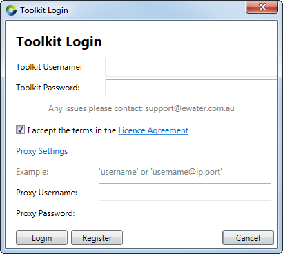
When you open Source for the first time, you will be prompted to enter your Toolkit login credentials:
- Enable the I accept the terms in the Licence Agreement) checkbox;
- If you have a Toolkit account, enter your credentials and click Login;
- If you do not have a Toolkit account, enter the credentials you wish to keep and click Register; or
- Click Cancel to exit from Source.
You must also enter proxy settings if your computer is located behind a proxy and you are unable to login.
Figure 1. Toolkit Login
If you are unable to login due to firewall issues, an auto-generated bypass code allows you to work offline. In this case, the dialog shown in Figure 3 appears.
Figure 2. Toolkit Login, Connection error
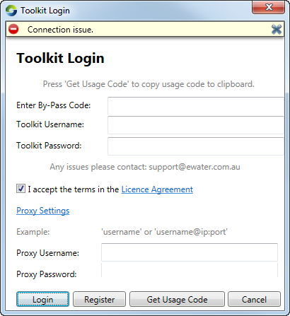
Follow these steps to generate a bypass code in this dialog:
- Enter your toolkit credentials in their respective fields and click Get Usage Code; This copies a code (called the Usage code) to your computer's clipboard and opens your browser to a Toolkit webpage;
- Carry out the steps outlined in Figure 3. Note that you will need a working network connection to access this website;
- Copy the bypass code generated in the Toolkit website (Ctrl+C) and paste it in the Enter By-pass Code field in Figure 2;
- Click Login to start using Source.
Figure 3. Toolkit website, bypass code
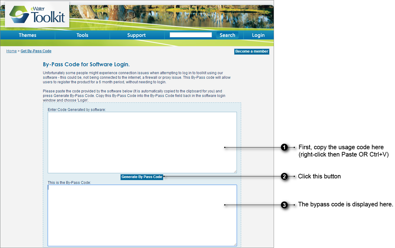
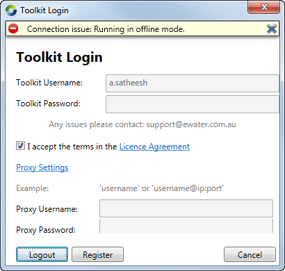
Figure 4. Toolkit Login, Offline
Once logged in, the Source splash screen (Figure 5) appears, which provides shortcuts to various actions in Source, including:
- Creating new projects and scenarios. The commands found here are synonyms for File New » Project... and File New Scenario..., and New Scenario on the File toolbar;
- Opening recent projects. You can also find a list of recent projects at File [recent documents]
- Finding more information about Source capabilities, news and release notes; and
- Accessing user guides and links to online training and other useful materials.
Additionally, you can report a bug and provide feedback by clicking on Report Bug/Feedback. Note that you must have a working Internet connection for this to work.
Figure 5. Source splash screen
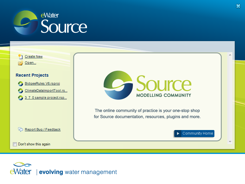
To skip the splash screen altogether and go directly to the main screen next time Source is launched, untick the Don’t show this again checkbox at the bottom left of the screen. To re-activate this option, select from the main interface, which will open the Welcome screen when Source is launched. Use the Don’t show this again checkbox on the bottom left corner to toggle the display of this screen.
Main screen
Once open, you can see that Source follows the user interface conventions of a standard Microsoft Windows™ application (shown in Figure 6). For example:
- The main window can be maximised or minimised using controls at the right hand end of the title bar;
- A menu bar with familiar File, Window and Help menus, with additional menus directing users to more specific functions of Source; and
- Toolbars providing point-and-click access to many commands.
The individual menus and toolbars, along with the commands they contain, are explained in more detail in the User interface reference chapter.
Figure 6. User interface for Source
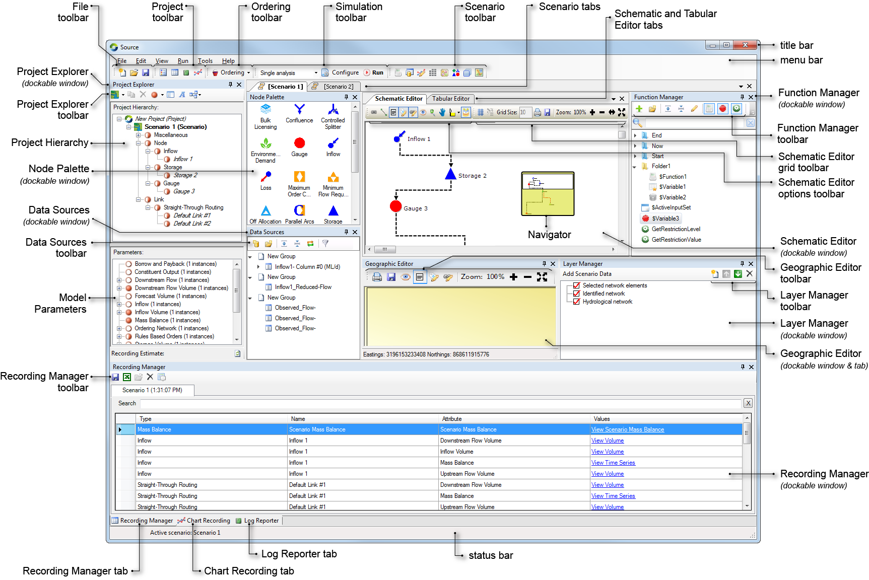
The following toolbars (available from the main Source screen) allow you direct access to various sections of Source (refer to the User interface reference for more information on these):
- Data Sources toolbar - allows you to add and manage sources of data (time series or by linking to another scenario). You can edit or view this data once it has been loaded in the Data Sources Explorer;
- File toolbar - contains commands for creating a new project, opening an existing project, and saving a project (and all the scenarios within that project);
- Function manager toolbar - allows you to add and manage all functions and expressions in Source;
- Ordering toolbar - provides quick access to ordering-related functions. The button on this toolbar reveals a pop-up menu;
- Project toolbar - allows you to hide or display the Project Explorer, Recording Manager, Log Reporter and Chart Recording Manager. To hide or display any of these windows, click the relevant button in the toolbar;
- Recording Manager toolbar - allows you to manage results in the Recording Explorer;
- Simulation toolbar - allows you to set the analysis type (single, stochastic or flow calibration), specify start and end dates for the simulation, and to run the catchment model; and
- Scenario toolbar - allows you to hide or display the Geographic Editor, Schematic Editor and Tabular Editor, the Function Manager, Data Sources, the Node Palette, the Layer Manager and Location Control panels.
Quitting Source
You can quit Source by doing either of the following:
- Choose ; or
Press Alt+F4 on your keyboard.
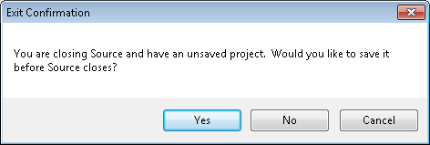
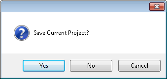
You are reminded to save your project (Figure 7). Click Yes to save your project and then quit, No to quit without saving your project, or Cancel to return to Source.
Figure 7. Exit confirmation
Creating a new project
To create a new project, do one of the following:
- Choose ;
- Click New Scenario on the File toolbar; or
- Press Ctrl+N on your keyboard.
You can only have one project file open at a time. Do not try to open the same project file using more than one copy of Source because you may lose your work.
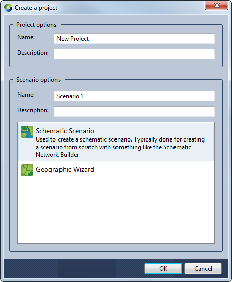
In the resulting window (Figure 8), enter the following:
- The project name. Give it a meaningful name or accept the default;
- The scenario name. Once again, provide a meaningful name or accept the default. All the scenarios in a project must have unique names;
- Choose the desired kind of scenario (refer to About scenario types for the different types available); and
- Click OK.
Figure 8. New Project dialog
Closing an open project
To close an open project, choose . This closes the current project and prompts to save your work (Figure 9). Click the appropriate button.
Figure 9. Close project
Opening an existing project
You can also open an existing project by doing one of the following:
- Choose or
- Click Open Project on the File toolbar.
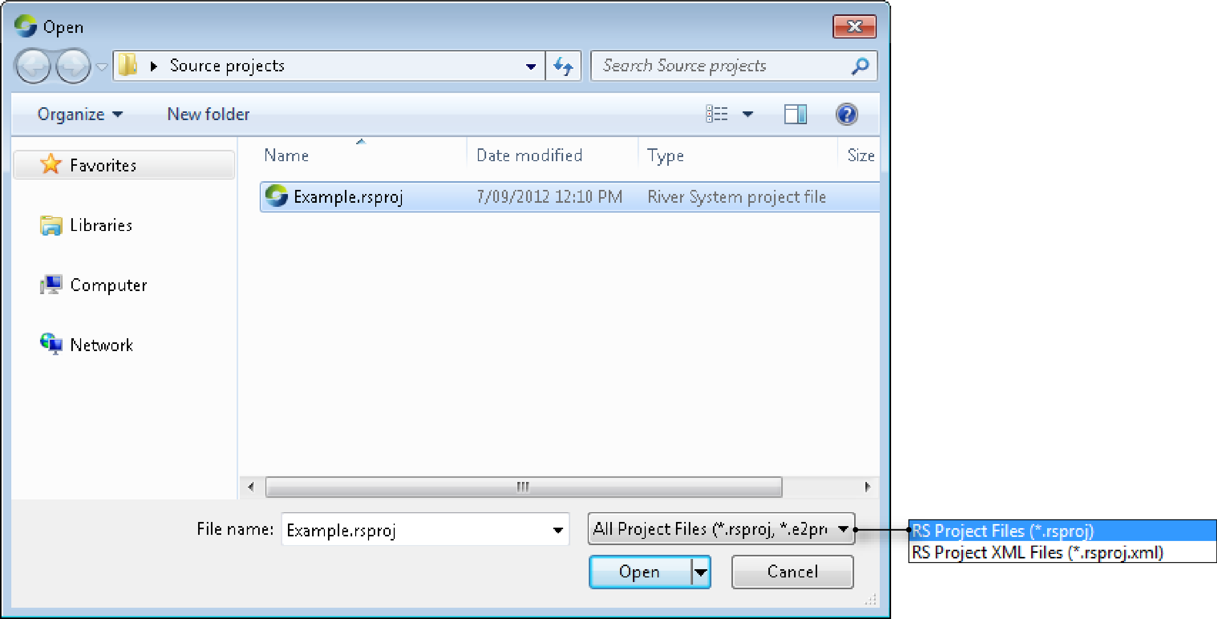
This opens the standard Windows™ open dialog (Figure 10). Note that opening a new project prompts you to save any open project.
Figure 10. Open project
About scenario types
Three scenarios have been described in this guide:
- A management scenario is primarily concerned with modelling longer time-scales;
- An operations scenario is primarily concerned with shorter time-scales. It utilises facilities for forecasting and working with unaccounted differences, and typically makes heavy use of the Tabular Editor; and
- A catchments scenario which deals with the management of upland catchment processes. It is usually constructed using the Geographic Wizard for catchments which is a structured sequence of steps that guides you through the construction process.
It is important to choose the correct type of scenario before you start building your model. Although a project can contain several scenarios, a scenario type is fixed once it is created and cannot be changed later. Note that scenarios are independent of each other. A change in one scenario does not impact another scenario.
Creating a scenario
A project must contain at least one scenario. Whenever you create a new project, you are also prompted to create a scenario. You can create additional scenarios using any of the following methods:
- Choose
- Click New Scenario on the File toolbar; or
- Click New Scenario (by menu) on the Project Explorer toolbar.
To create an Operations scenario, first create a River Manager scenario. Then, choose Tools » Rivers Operations
Opening a scenario
When a project only contains one scenario, that scenario is opened automatically when you open the project. However, when a project contains more than one scenario, you must open each scenario individually.
To view a scenario that is contained within a project, double click the scenario name from the list in the Project Hierarchy. This opens the appropriate editor for the selected scenario, and changes the scenario name to a bold appearance so that you know it is the current, or active scenario.
You can also select a scenario from the list of loaded scenarios on the View menu. Selecting a scenario from the list makes it active.
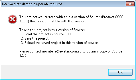
You can only open a project that was created in an older version of Source if it was originally created in v3.1.0. If it was created in an earlier version, an error message (Figure 11) will appear prompting you to open the project in v3.1.0, save it, then re-open it in the working version. When you re-open it, you will be prompted to save a backup of your project after which your project will be upgraded automatically to the current version of Source.
Figure 11. Opening a project, error
Copying a scenario
You can duplicate existing scenarios. You may want to do this if you wish to experiment with variations without affecting your original scenario.
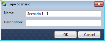
To copy a scenario, click Copy Scenario on the Project Explorer toolbar. Source makes a copy of the current scenario and asks you to name the copy (as shown in Figure 12). You can either accept the proposed name or supply one of your own. Keep in mind that scenario names must be unique within a project.
The new (copied) scenario will be a duplicate of the original at the time of the copy.
Figure 12. Copy Scenario
Renaming a scenario
Source automatically gives new scenarios the default name of "Scenario #n" , where n is a number. To rename a scenario:
- Select the scenario in the Project Hierarchy; and
- Once the scenario name is selected, pause then click again. When the entry is highlighted, you can enter a new name. Remember that scenario names must be unique within a project.
Saving your work
Save your work by doing either of the following:
- Choose
- Click Save Project on the File toolbar.
If you have not saved your project previously, choose and you will be prompted to name your project (Figure 13). Source uses the Windows file extension ".rsproj" or ".rsproj.xml" to identify its project files. Saving a project automatically saves all the scenarios stored within the project.
Figure 13. Save project
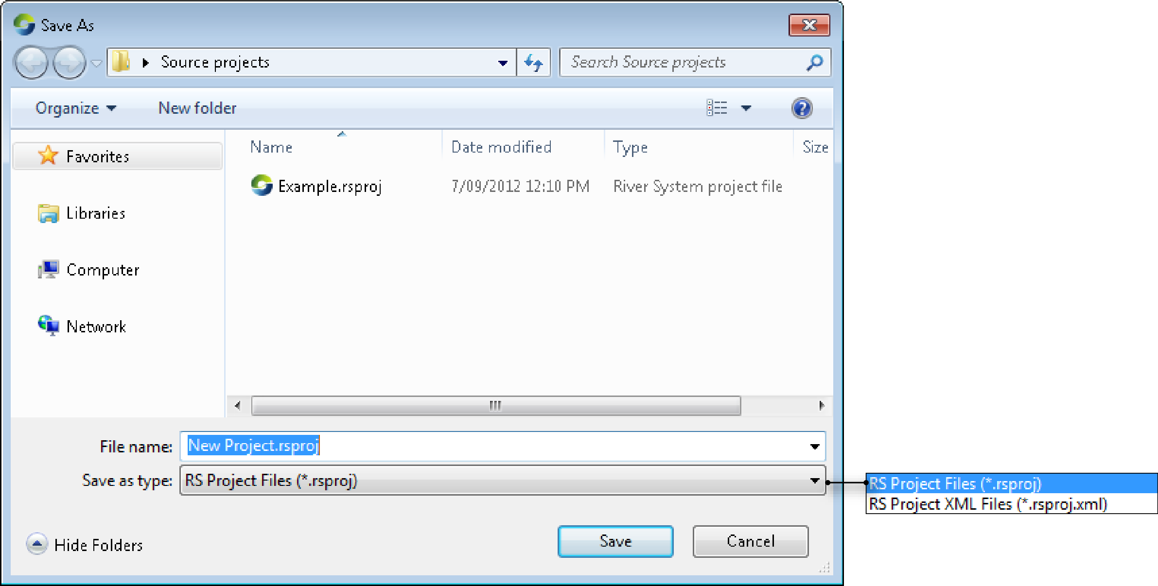
If you save a project in the folder where Source is installed, the project may be removed during an un-install procedure.
Editors
Source uses editors which are tailored to the needs of the main scenario types. There are three main editors, known as the Geographic, Schematic and Tabular editors, which support the catchments, management and operations scenario types respectively. These editor-scenario type associations are not absolute and you will often use multiple editors within a given project. For example, you can use the Schematic Editor to define the model of a river system for both operations and management scenario types. Details for each of these editors are available at Geographic Editor, Schematic Editor and Tabular Editor.
Project Explorer
The Project Explorer (Figure 14) allows you to manage model components using a combination of the menu bar, the Project Hierarchy, the Model Parameters area, and pop-up menus. For an active scenario, clicking an item in the Schematic or Geographic Editor highlights it in the Project Hierarchy.
Figure 14. Project Explorer
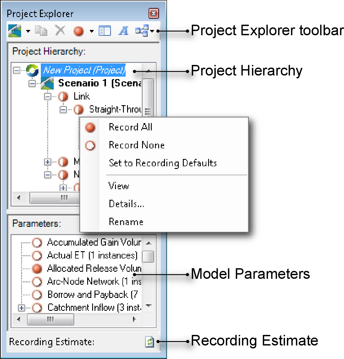
Project Hierarchy
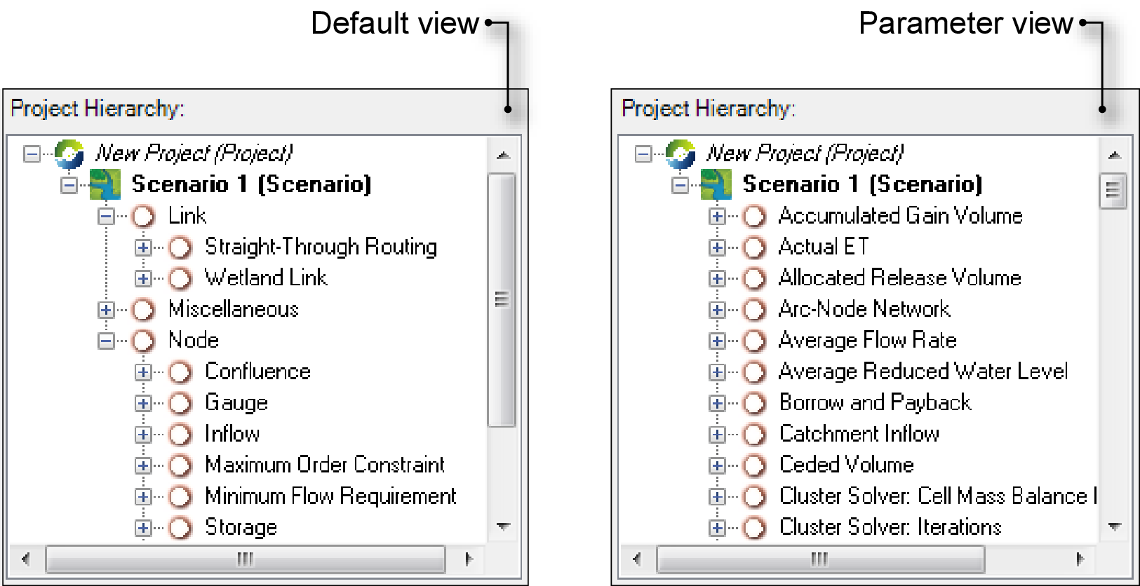
The Project Hierarchy (refer to Figure 14) displays a structural breakdown of the project. The type of display will depend on the view selected within the View Type pop-up menu on the Project Explorer toolbar. All view options will display at least the project and scenarios within the project. The Default View, which is shown on the left side in Figure 15, displays individual elements that make up a model. The Parameter View (right side in Figure 15) displays all the recordable parameters for the model.
Figure 15. View type menu options
Model parameters
The Model Parameters area (refer to Figure 14) shows which parameters will be recorded for the scenario element (node, link, catchment etc) that is currently highlighted in the Project Hierarchy. The indicators have the following meanings:
 Every parameter at this level and below will be recorded; or
 No parameters at this level and below will be recorded.
 Some (but not all) parameters at this level and below will be recorded.
To change which parameters are recorded, first select an element in either the Project Hierarchy or Model Parameters area, then use either the Recording Options pop-up menu on the Project Explorer toolbar, or the contextual menu to change the setting. Note that these commands are hierarchical in nature and affect both the selected element and its logical children as displayed in the visual hierarchy. You can also define a set of default recording options to be applied to all of your projects. See Recording Manager defaults.
Data Sources
The Data Sources tab allows you to view and manage time series at one location in Source. When time series are added using the Data Sources Explorer, they are available for use throughout Source. For more details on using this, refer to Importing data.
Function Manager
The Function manager panel allows you to create, manage and maintain all functions and expressions defined in Source. Just as all data in the Data Sources Explorer is available throughout Source, all functions and expressions added in the Function manager can be used in the same way.
Node Palette
The Node Palette contains a list of icons representing the nodes that are supported by Source. To create a node-link network, drag icons from this palette onto the Schematic Editor’s drawing surface.
Layer Manager
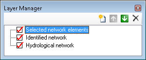
The Layer Manager (Figure 16) is mainly associated with the Geographic Editor. It is visible by default when you create a new catchments scenario. Choose if the Layer Manager is not visible. You can add new layers, and move layers up and down in order of visibility. The checkbox next to a layer’s name indicates that the layer is visible in the Geographic Editor. Note that any layers that are added or removed are not persisted in the scenario.
Figure 16. Layer manager
Recording Manager
The Recording Manager displays a list of all the recorded results from the model run or runs. Each model run has its own tab. You can sort the results by clicking the column headings. The associated with this window gives quick access to common functions.
Log Reporter
The Log Reporter displays any errors, warnings or information messages resulting from user actions, or events that have occurred when running a scenario. You can choose to display or hide different types of events by clicking the Errors, Warnings, or Info tabs at the bottom of the Log Reporter.
Chart Recording
Chart Recording allows you to compare the results of different scenario runs. You can change certain parameters in a scenario to see how the output is affected. Refer to Chart Recording Manager for more information on this.
Dockable windows (This is not operational in Source 3.7.0)
Many Source windows can be docked within the main window, or arranged independently. The dockable windows include the Geographic, Schematic and Tabular editors, most of the auxiliary windows, and windows belonging to some plugins. The docking and undocking action sticks with a project and scenario when it is saved. If the Schematic Editor is not docked, and a project is saved and closed, when it is re-opened, the Schematic Editor will be in the same position it was when the project was closed. The same applies if Source is closed and re-opened.
Undocking windows
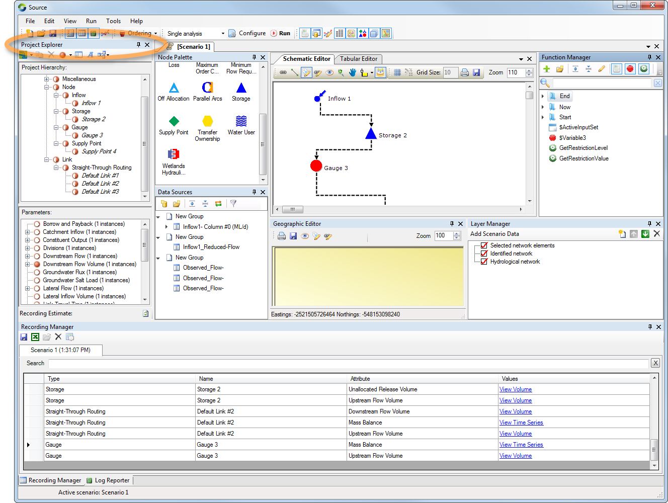
The default position of dockable windows is docked. A single click within the borders of any docked window will activate it. An active window can be identified from either its title bar or from an element within it that is highlighted. For example, the Project Explorer is the active docked window in Figure 17.
Figure 17. Identifying active windows
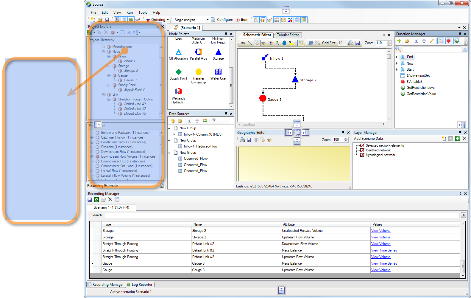
You can undock a window by dragging its title bar to a new location (eg. Figure 18). This can be into another docked position within the main window, or to a position outside the main window. The predicted position of a window is indicated by a transparent outline. When you release the mouse button, the window will be placed in that position. You can also double-click a docked window’s title bar to undock it. The remaining windows will reposition to take up any vacant space within the main window.
Figure 18. Window undocking (highlight)
Undocking plugin windows
The windows of some plugin tools (eg.GWLag) may be docked in the main window. However, once a plugin window has become docked, the window has no title bar which can be dragged or double-clicked to cause it to become undocked. You can undock such a window by:
- Re-choosing the menu command that you used to open the window. This will cause the associated window to become undocked; or
- Choosing . This will do as the name suggests and reset all windows to their default arrangement. For plugins, the default state is that the window is closed.
Docking windows
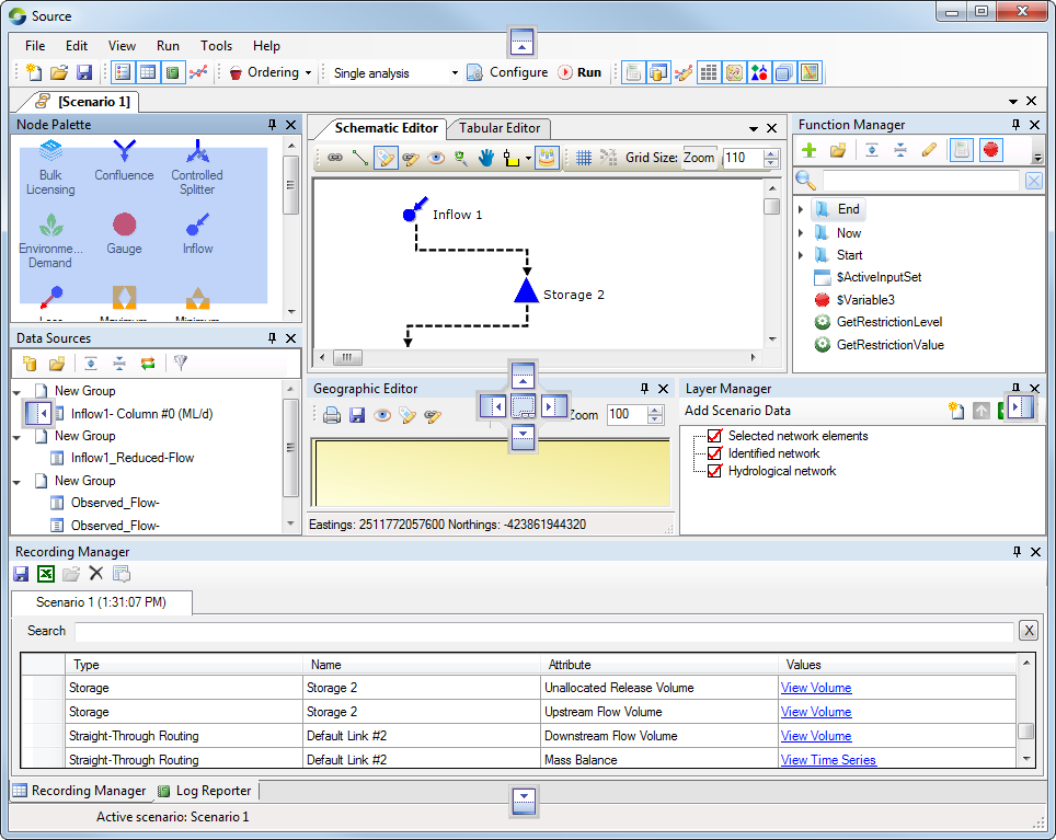
You can dock an undocked window within the main Source window by dragging it back into the main window. Source highlights potential target locations with transparent outlines (Figure 19). Choose the desired position and release the mouse. You can also re-dock an undocked window by double-clicking its title bar. The window will become docked in the main window, usually in the position it occupied before it was last undocked. The other docked windows will resize to accommodate the incoming window.
Figure 19. Window docking
Auto-hiding dockable windows
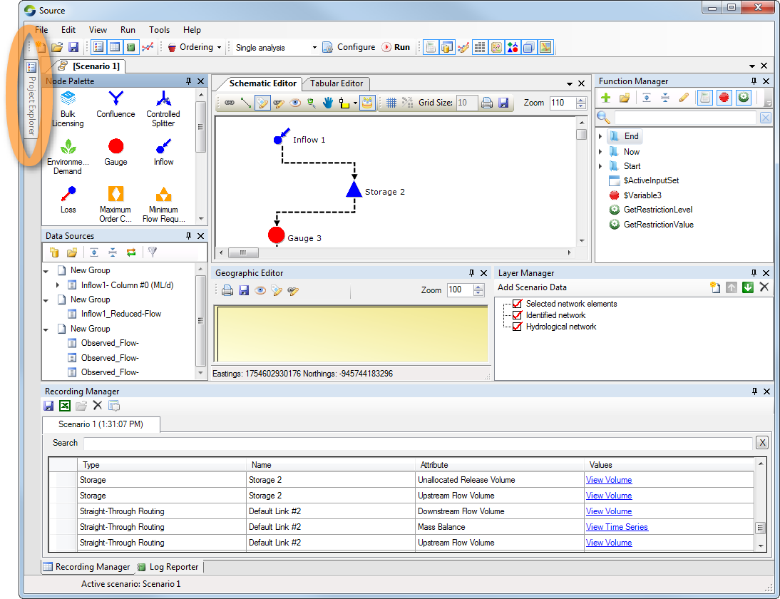
Many of the dockable windows can be hidden temporarily to allow for improved use of screen space. To activate the auto-hide function, click the  icon at the top right hand corner of the window you want to auto-hide. The icon turns 90° to indicate that the window is in auto-hide mode and the window reduces to a tab at the side of the main window (Figure 20). You can inspect a hidden window by hovering the mouse pointer over its tab. The hidden window will slide open and will remain open while the mouse pointer remains within its borders. When you move the mouse pointer beyond the window’s confines, it will slide closed. If you click anywhere inside a hidden window, it will remain open until you click beyond the window’s confines.
Figure 20. Window auto-hiding (tab display)
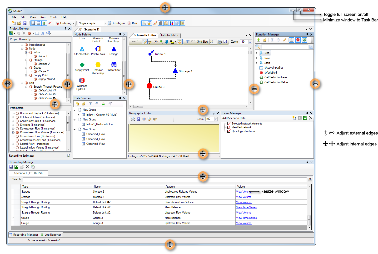
Adjusting window sizes
The overall size of the main window can be adjusted using a combination of the full-screen toggle (Maximize) and Minimize controls, the window Resize control, and/or by dragging the four edges of the window. Within the main window, the amount of space taken by each docked window can be adjusted by dragging the split window controls. All of these controls are shown in Figure 21. The controls to drag internal and external window boundaries only become available when the mouse cursor is placed over the critical regions. Once the cursor changes to an edge-dragging control, click and hold the mouse cursor, then drag the cursor in the appropriate direction to adjust the window edge.
Figure 21. Window size adjustment controls
About feature editors
A feature editor window allows you to define various parameters for nodes and links. It opens when you double click on components in the Schematic Editor. You can also open a feature editor by right-clicking on the node or link and choosing Edit from the contextual menu.
Each node or link type supports different parameters, so the exact structure of feature editors varies according to the type of node or link being manipulated. However, the controls shown in Figure 22 are common to many feature editors.
The left panel lists all parameters associated with the node or link. You can also add a note to a node or link to indicate a specific feature for example, which may affect its behaviour during a scenario run. This note is indicated as an exclamation mark on the component's icon in the Schematic Editor. It also appears in the Recording Manager after a scenario run. To include a note, right click on the component's icon in the feature editor and choose Add Note. This is shown in Figure 25.
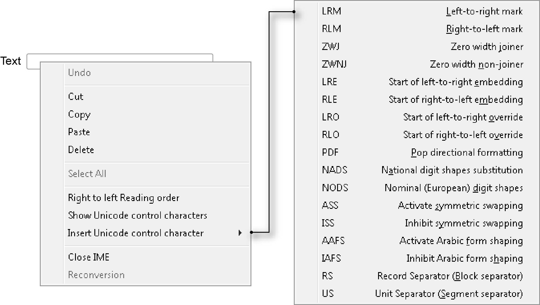
Contextual menus can be accessed by right-clicking on various elements in the user interface. In some cases, choices in contextual menus duplicate those in toolbars and the main menu structure. In others, the contextual menus are the only way to access a particular function. All contextual menus available in Source are shown with the relevant feature editor or graphic;
Figure 22. Feature editor (common controls)
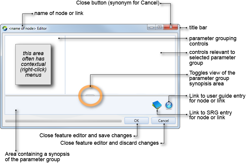
Figure 23. Text field contextual menu
Other behaviour which is shared by a number of feature editors includes:
- Parameters applicable to a node or link may be grouped according to related purposes;
- Some user interface elements are only enabled if their prerequisites have been met;
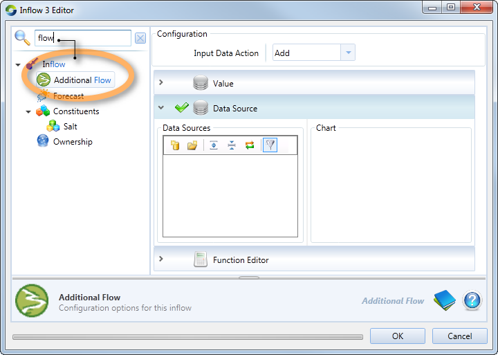
- The ability to search for elements in the hierarchical list, with the result displaying all instances of the query (both parent and child if applicable). Notice that when you enter the search criteria (as shown in Figure 24), the results are displayed in blue. In this case, the term ‘flow’ appears in both the parent and child; and
- When multiple values can be entered for a single parameter, only one value can be adjusted at a time. A highlight (normally blue) indicates the field being manipulated. To edit a different field in this table, click the mouse pointer in the target field.
Figure 24. Inflow node (Search functionality)
Many feature editors support loading parameter information from a file. Where present, the Import... button can be used to load parameters into a feature editor whereas the corresponding Export... button will save the table’s current values to an external file. Additionally, as an alternative to entering or importing discrete parameter settings, the feature editors for many nodes allow for the node’s behaviour to be defined via an arithmetic expression or function (refer to Working with the Function manager).
About notes
You can include a text based message associated with a node, link or function, which can be either:
- Informational;
- Warning; or
- An error.
To add a note to a node or link, refer to Adding notes to nodes and links. For functions, refer to Adding a note to a function.
Each of the different message types has a different icon. Figure 25 shows an example of an informational note added at an Inflow node.
Figure 25. Notes, Overview

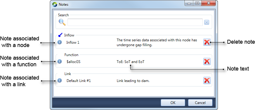
A summary of all nodes configured in a scenario can be viewed using View » Notes. This opens the Notes dialog (shown in Figure 26) displaying all the notes that have been configured. In this example, the Inflow1 node, the $allocGS function and the Default Link #1 link have notes associated with them.
Figure 26. Notes, Summary
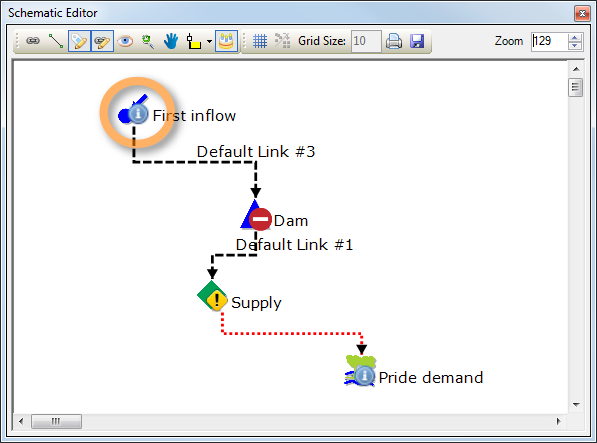
Once all the notes have been added and the scenario has been run, the Schematic Editor shows all the nodes that have notes configured on them. Figure 27 shows nodes with two informational notes, one warning, and one error note.
Figure 27. Schematic Editor, Notes on nodes
About piecewise linear editors
Piecewise linear editors are used in a number of places within Source. They allow you to arbitrarily define complex relationships in two dimensions. A typical use is a relationship between inflow (on the X-axis, or abscissa) and outflow (on the Y-axis, or ordinate). As the name suggests, piecewise linear editors are formed by concatenating line segments. The number of coordinate-pairs entered into any piecewise linear editor, and the comparative simplicity or complexity of the resulting relationship "curve", is up to you.
In most cases, piecewise linear editors adhere to the following constraints and conventions:
- The origin is (0,0) and there is no need for extrapolation in the negative direction along the X-axis. If (0,0) is missing from the data set, it may be assumed;
- Interpolation can be used to extrapolate the Y-value for any intermediate X-value;
- The right-most line segment projects linearly to infinity and can be used to extrapolate the Y-value for any X-value along that line. One exception to this rule occurs in the case of BigMod flow routing where the Y-value corresponding with the largest value of X in the table is used for all larger values of X (ie, the data points in the table are treated as though they define the left-hand edge of a histogram bar); and
- Mass balance is respected. For example, losses cannot exceed inflows, so all loss values are clipped to inflows. Similarly, negative volumes are untenable so any projection returning a negative number will also be clipped to zero.
In general, you will avoid problems if you adhere to the following guidelines:
- You should always include an explicit origin of (0,0). This avoids the need for the model to extrapolate in the negative direction along the X-axis. It also avoids any potential problems which might arise if the model silently assumes an origin of (0,0);
- X-values should always be in monotonically increasing order. In the current implementation, an X-value that is entered out of order is highlighted in red until a Y-value is entered, after which Source re-orders the table. You can use this feature to add interstitial coordinates to a table by adding new (X,Y) coordinates to the last row and waiting for the table to re-order;
- Y-values should also increase monotonically. Be cautious if you need to violate this guideline, and especially cautious if the right-most line segment has a negative slope;
- The right-most coordinate pair should lie beyond your most extreme known value. This avoids the need for the model to extrapolate in the positive direction along the X-axis, and also means that you do not need to remember which piecewise linear editors use linear extrapolation of the right-most line segment vs those which project the right-most Y-value to infinity;
- All values should be sensible. For example, there is no point in entering coordinate-pairs that violate mass balance (eg. a loss exceeding inflows); and
- If your model employs optimised ordering, keep your piecewise linear editors to as few data-points as possible. Complex curves usually increase run-time and can sometimes lead to infeasible solutions. Refer to the chapter on Ordering.
Working with date-pickers
Date-pickers are used in a number of places within Source. They are a combination of an editable text field and a pop-up calendar. Figure 28 shows the relationship between the various components.
Figure 28. Date-picker
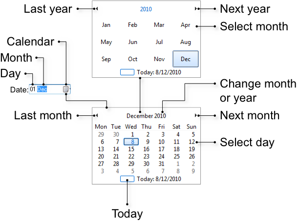
You can edit a date directly by selecting either the Day, Month or Year element within the text field (you cannot select the day of the week). Once an element has been selected, you can also change the selection by using the left and right arrow keys. You can adjust an element’s value by using the up and down arrow keys or by entering a new numeric value. Note that you also use numeric values for the Month element. For example, typing "7" changes the Month element to "July".
Clicking the disclosure arrow at the right of the text field displays a calendar. Within the calendar, you can:
- Change the month, year, decade or century by clicking repeatedly on the current year field;
- Change the month using the Last month and Next month buttons;
- Change the selected date using the arrow keys. The left and right arrow keys adjust the date by one day at a time whereas the up and down arrow keys adjust the date by one week at a time; and
- Select a date by clicking on the day. You can also select "today" by clicking the unnamed button at the lower, left of the calendar.
Selecting a date, pressing return, or clicking outside of the calendar’s confines closes the calendar.