Links
Links connect nodes in Source - they link, store and route water passing between nodes. You can only connect nodes using links and you cannot connect two links to each other without an intervening node.
A reach refers to a stretch of river, or physical section, between an upstream and downstream location. A link, on the other hand, is a logical connection within a river systems model. Routing describes the change in timing and shape of flow as water moves down a river.
Links (or reaches) can have routing configured on them. For links (or reaches) that do not have routing configured, they are used to define the order of execution in the model.
Using links in Source
You can configure some aspects of links in a similar way to nodes. Refer to Renaming nodes and links, Searching for nodes and links, Deleting nodes and links, Node and link default names and Copying and pasting.
Adding links to a model
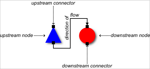
There are two types of links available depending on the nodes you are connecting (refer to Figure 1).
Vertical links are used to connect most nodes. To add this link to a model, first refer to Figure 1 which defines the terminology. To create the link:
- Position the mouse cursor over the upstream node;
- Click and hold on one of its downstream connectors and start dragging;
- When you start dragging the mouse cursor, candidate targets are displayed (as large icons) for the upstream connector of a downstream node; and
- Release the mouse and the link will ‘snap’ into place.
Figure 1. Node connection terminology
Horizontal links (or wetland links) are drawn between the Wetlands Hydraulic Connector node (source) and the Storage node (target) only. This process is similar to drawing a vertical link. Note that the node connectors appear on the left and right side, instead of above and below the nodes. Click and drag these connectors together as described for vertical links. Figure 2 shows an example of a horizontal link.
Figure 2. Horizontal link

You can also drag the link vertically once it has been created by clicking on the red dot. This appears in the centre of the link when you click on the link. For more detail on the wetland link, refer to Wetland Link.
Dragging links
You can disconnect and reconnect a link between nodes rather than having to delete and re-add it using the Allow Link Dragged button in the Schematic Editor options toolbar. Note that not all links can be connected to all types of nodes, and specific nodes require certain links. Refer to Types of link routing for more detail.
Editing link parameters
To edit link parameters using a feature editor, refer to About feature editors.
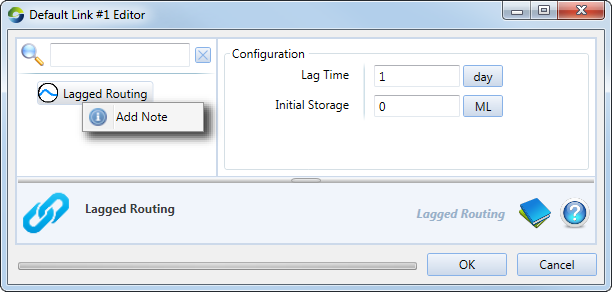
Adding notes
You can include a text-based message, or note, for a storage routing link. Refer to Adding notes to nodes and links for details.
Link elevation
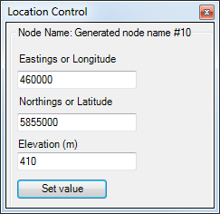
You can set the elevation for a link using the Location Control window (shown in Figure 3). Choose View » Location Control to open this window.
Figure 3. Location Control window
Types of link routing
Source supports three types of link routing. You can either use straight through routing, a lagged routing model or a storage routing model. To enable routing, right click on the link, choose Routing Type, then click on the required link routing.
A demand link is created when you connect a water user node to a supply point node, and is represented in the Schematic Editor using dashed red lines. They behave like no routing links and cannot be configured.
A wetland routing link interconnects wetland hydraulic connector nodes and/or storage nodes. A wetland link is also known as a horizontal link because it is can only attach to the sides of storage and wetland connector nodes, rather than their upstream or downstream connectors. The presence of a horizontal link at a storage node indicates that the storage is behaving as a wetland. A wetland routing link is represented in the Schematic Editor as a solid green line with an arrow representing the expected direction of flow, which is set when you draw the link.
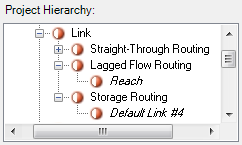
Figure 4. Project Hierarchy (link models)
Straight through routing
All links are assigned straight through routing by default. This link has the following features:
- Water enters and exits such a link in the same time-step;
- There are no configuration parameters associated with straight through routing links; and
- You cannot configure fluxes, constituents or ownership.
Straight through routing links are represented in the Schematic Editor using black, dashed lines.You can check which routing models are in use in a scenario using the Project Hierarchy. The example in Figure 3 shows that both lagged flow and storage routing are in use. You are responsible for ensuring that you use the correct model for each link.
Lagged flow routing
Lagged flow routing only considers the average travel time of water in a river reach. It does not consider flow attenuation The flow entering a link exits that link at some whole number of time-steps in the future. This type of link is represented in the Schematic Editor as a black line, with alternating dots and dashes. Once you have enabled lagged flow routing, double click the link to configure the settings.
Figure 5. Link (Lagged flow routing)
Lag Time represents the time it takes for water to travel along the link and is a positive real number. Initial Storage is the amount of water deemed to be in the link on the first time-step. For example, if there is a lag of two days, and there is 10ML in the link at the start of the run, then 5ML is deemed to be flowing out each day (total initial storage divided by lag).
Travel time in the reach is computed as follows:
| Equation 1 |  |
|---|
A link configured for lagged flow routing is treated as a series of sub-reaches of equal length, with the travel time in each sub-division equal to one time-step. Water moves through the link progressively, without attenuation. You cannot configure fluxes, constituents or ownership on a lagged flow routing link. If lateral flows are significant and/or there is dead storage in the reach, you can approximate lagged flow routing using generalised non-linear storage flow routing, as follows:
- Compute the number of divisions, n, by dividing the average wave passage time by the model time-step and round the result to a whole number. The result must be at least one (ie n ≥ 1).
- Configure a storage flow routing reach where:
- n = number of divisions;
- x = 1;
- m = 1; and
- K = model time-step.
- If you need to account for lateral flows where n=1 and the average travel time is a fraction of the model time-step (eg. a reach with a one day lag in a model with a monthly time-step), you can adjust K to a smaller value without affecting the shape of the hydrograph.
Storage flow routing
This type of link is represented in the Schematic Editor as a solid black line. Storage routing is based on mass conservation and the assumption of monotonic relationships between storage and discharge in a link.
The stability criteria must also be satisfied for a model to run correctly. If this is not the case, the following error appears during runtime: Routing parameters have caused instability in storage routing. Refer to Stability criteria for more information.
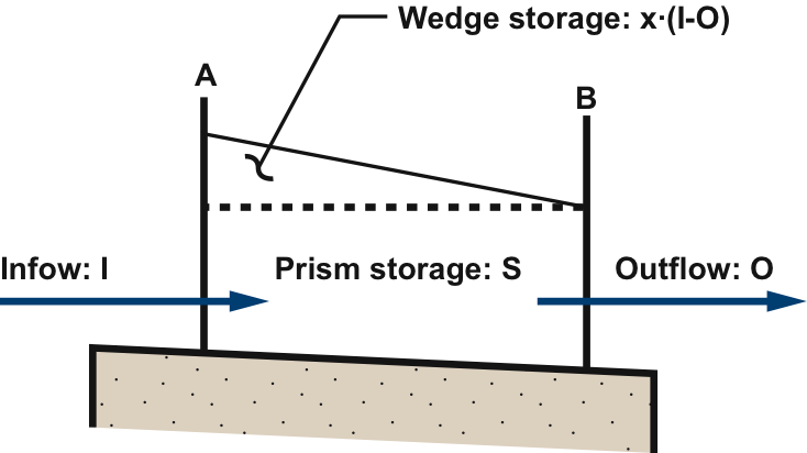
This is a simplification of the full momentum equation and assumes that diffusion and dynamic effects are negligible. The method uses index flow in flux, storage and mass balance equations. A weighting factor is used to adjust the bias between inflow and outflow rate, hence allowing for attenuation of flow. The storage routing equation is shown below and some of its terms are represented diagrammatically in Figure 6:
| Equation 2 | 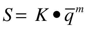 |
|---|
where:
S is the storage in the reach,
K is the storage constant,
m is the storage exponent, and
q‾ is the index flow, which is given by
| Equation 3 | 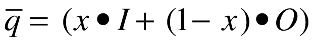 |
|---|
where:
I is inflow to the reach during the time-step,
O is outflow from the reach during the time-step, and
x is the inflow bias or attenuation factor.
Figure 6. Prism and wedge storage
Refer to the Source Scientific Reference Guide for more details.
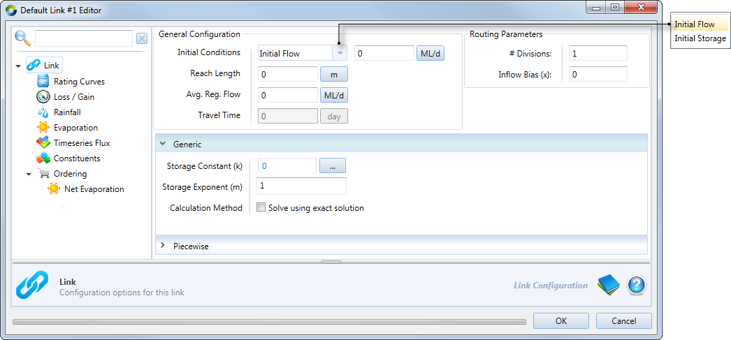
Figure 7 shows the parameters required to configure storage routing on a link.
Figure 7. Link (Storage Routing), Generic
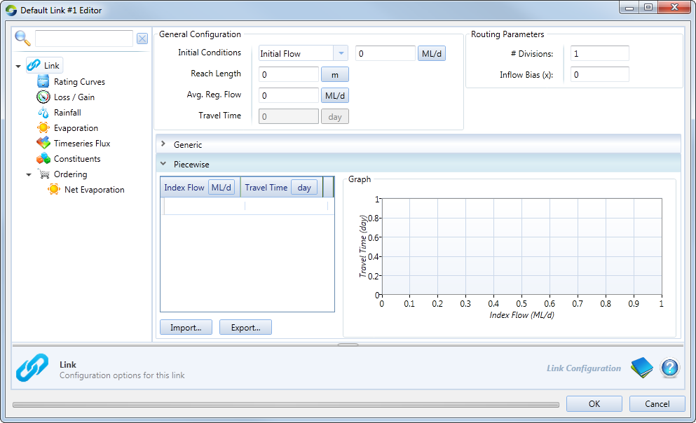
You can also specify a piecewise relationship (as shown in Figure 8) instead of a generic one.
Figure 8. Link (Storage routing), Piecewise
About dead storage
Dead storage refers to the capacity of a storage that is below the minimum operating level. At this water level, there is no outflow. The level of the reach with respect to dead storage at the beginning of the time-step affects its level in subsequent time-steps as follows:
- The reach is at or below dead storage and the fluxes during the time-step are insufficient to raise the level above dead storage; or
- The reach is above dead storage but fluxes during the time-step would lower the level in the reach to below dead storage; or
- The reach is above dead storage and remains above dead storage during the time-step.
To determine if the reach is at or below the dead storage level, Source:
- Computes an initial storage estimate by using inflows to fill the reach up to but not exceeding the dead storage level;
- Computes a revised storage estimate based on any remaining inflows and fluxes but ignoring outflows; or
If the revised storage estimate is above dead storage then outflows are computed, otherwise the initial storage estimate is used and outflows are set to zero.
The next section provides an overview of the parameters shown in Figure 5.
Initial conditions (flow or storage)
If necessary, one of these parameters may be used to seed a reach with either an initial flow or storage so that reach behaviour is fully defined from the first model time-step.
Reach length
The Reach Length is not used in computations and is only for documentation purposes.
Average regulated flow
This parameter is used to calculate travel time for orders in the ordering phase. It is not used in the flow distribution phase.
Number of Divisions
Conceptually, this parameter describes the number of times that a reach is replicated. The effective length of a reach is determined from its behaviour, which is controlled by the combination of the storage exponent m, the inflow bias x and the storage constant K. Specifying multiple reach divisions implies applying the same set of behavioural parameters multiple times. In other words, if the effective length of a single-division reach is 500 metres (as derived from its behavioural parameters), changing the # Divisions parameter to 2 implies a combined effective length of 1000 metres. If you want to sub-divide a 500 metre reach into two 250 metre sections, you must also change the behavioural parameters to achieve this.
Inflow bias
The weighting factor x is used to adjust the bias between inflow and outflow rate and allows for flow attenuation. A recommended starting value is 0.5.
Storage exponent
If m=1, linear (Muskingum) routing is implied, otherwise non-linear routing is implied. A recommended starting value for non-linear routing is m=0.8. Laurenson routing is obtained when m≠1 and x=0, in which case the storage routing equation simplifies to:
| Equation 4 | 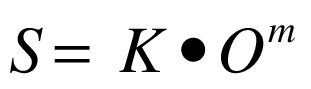 |
|---|
Storage constant
When using linear routing (m=1), the units of the storage constant K are in seconds. For models using daily time-steps, the recommended starting value is 86400 (the number of seconds in one day). When using non-linear routing (m≠1), the recommended starting value should be calculated as follows:
| Equation 5 | 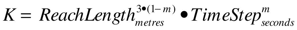 |
|---|
For example, if the reach length is 1000 metres, the time-step is one day, and m=0.8:
| Equation 6 |  |
|---|
The parameters for storage flow routing are summarised in Table 1.
Table 1. Link (Storage routing parameters)
| Parameter | Units | Range | Default |
|---|---|---|---|
| Initial flow | megalitres per day | real ≥ 0 | 0 ML/d |
| Initial storage | megalitres | real ≥ 0 | 0 ML |
| Reach length | metres | real ≥ 0 | 0 metres |
| Average regulated flow | megalitres per day | real ≥ 0 | 0 ML/d |
| Number of reach divisions | whole units | integer ≥ 1 | 1 |
| Inflow bias (attenuation factor, x) | dimensionless | real 0 ≤ x ≤ 1 | 0 |
| Storage exponent (m) | time-steps | real 0 < m ≤ 1 | 0 time-steps |
| Storage constant (K) | K units | real ≥ 0 | 0 |
Piecewise storage function
Link travel time can also be set using a piecewise linear editor. This describes a series of relationships between reach index flow rate q¯ versus travel time. The slope of the curve is the same as that for index flow rate versus storage so the rating curve can be derived using dead storage (zero flow) as the starting point. The data points can be entered manually or imported from a .CSV file, the format of which is shown in Table 2. Quadratic interpolation is used to find points in each defined segment on the curve (as in BigMod where x=1).
Table 2. Link (Storage routing travel time, data file format)
| Row | Column (comma-separated) | |
|---|---|---|
| 1 | 2 | |
| 1 | Index flow (ML/d) | Travel time (day) |
| 2..n | flow | lag |
Piecewise routing allows you to specify how K varies with flow. If x=1 then K must always be less than or equal to the time-step. In BigMod routing, the highest value of K is found in the travel time relationship, and the reach should be subdivided into sufficient divisions such that the highest value of K for each division is less than half the time-step.
Link rating curve
Rating curves are used to describe the physical characteristics of the reach and convert a flow into a level, ie. they produce an output of level. The piecewise linear editor allows you to define relationships with respect to water level, discharge rate, reach width and dead storage. You can define multiple rating curves for a reach, each scheduled to commence on a particular date.
To define a new rating curve:
- Right click Rating Curve and choose Add Rating Curve;
- Today’s date will automatically be entered for Start Date. To change this, click the calendar on the right side (see Working with date-pickers);
- Enter the water level, discharge rate, reach width and dead storage; and
- Enter an appropriate value for Overbank Flow Level.
You can also use the Import button to import a rating curve from a .CSV file the format of which is shown in Table 3.
Table 3. Link (Storage routing, Rating curve, data file format)
| Row | Column (comma-separated) | |||
|---|---|---|---|---|
| 1 | 2 | 3 | 4 | |
| 1 | Level | Discharge (ML/d) | Surface width (m) | Dead storage (ML) |
| 2..n | level | rate | width | storage |
Where:
level is the storage height in the reach in metres above dead storage
rate is the outflow from the reach in megalitres per day in the corresponding level
width is the surface width of the reach in metres at the corresponding level
storage is the dead storage in the reach in megalitres at the corresponding level.
There should be at least one row describing the maximum depth at which there is zero flow, and which quantifies the maximum amount of dead storage in the reach. Thereafter, the dead storage volume should remain constant. Table 4 shows an example of this. A depth of 0.5 metres defines the maximum amount of dead storage (100 megalitres), after which the dead storage remains constant. Note that if discharge is 0, then dead storage must be increasing, or it must be equal to the previous value of dead storage.
Table 4. Link (Storage routing, Rating curve, example)
| Level (m) | Discharge (ML/d) | Surface width (m) | Dead storage (ML) |
|---|---|---|---|
| 0 | 0 | 0 | 0 |
| 0.1 | 0 | 5 | 50 |
| 0.5 | 0 | 10 | 100 |
| 1 | 10 | 11 | 100 |
| 5 | 500 | 15 | 100 |
To edit an exising rating curve, select the curve from the list of available curves under Rating Curve. Edit the data and click OK to close the editor. To delete a rating curve, right click the curve from the list and choose Delete.
You can also export rating curves to .CSV files by clicking the Export button. Table 3 shows the file format.
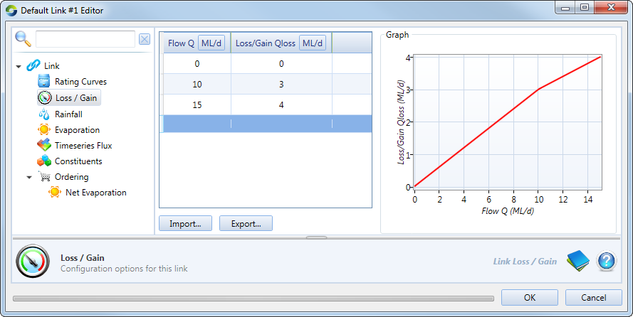
Link losses and gains
Choose Loss/Gain to specify flux as a function of flow using a piecewise linear editor.
By convention, losses are described using positive numbers whereas gains are specified using negative numbers. In other words, a gain is a negative loss.
Figure 9. Link (Storage routing, Loss/Gain)
You can enter the relationship manually, or import the data from a .CSV file, the format of which is shown in Table 5. This table shows the data file format for both evaporation and rainfall.
Table 5. Link (Evaporation.Rainfall, data file format)
| Row | Column (comma-separated) | |
|---|---|---|
| 1 | 2 | |
| 1..n | time | value |
Where:
time is the time of observation in "dd/mm/yyyy hh:mm:ss" format
value is the evaporation rate.rainfall in millimetres per time-step
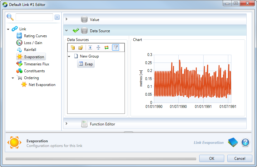
Link evaporation
Choose Evaporation to specify the rate of evaporation per unit of surface area. Typically, this is done using a time series (loaded using Data Sources), the format of which is shown in Table 5. You can also specify the rate of evaporation as a single value, or as an expression using the Function Editor.
Figure 10. Link (Storage routing, Evaporation)
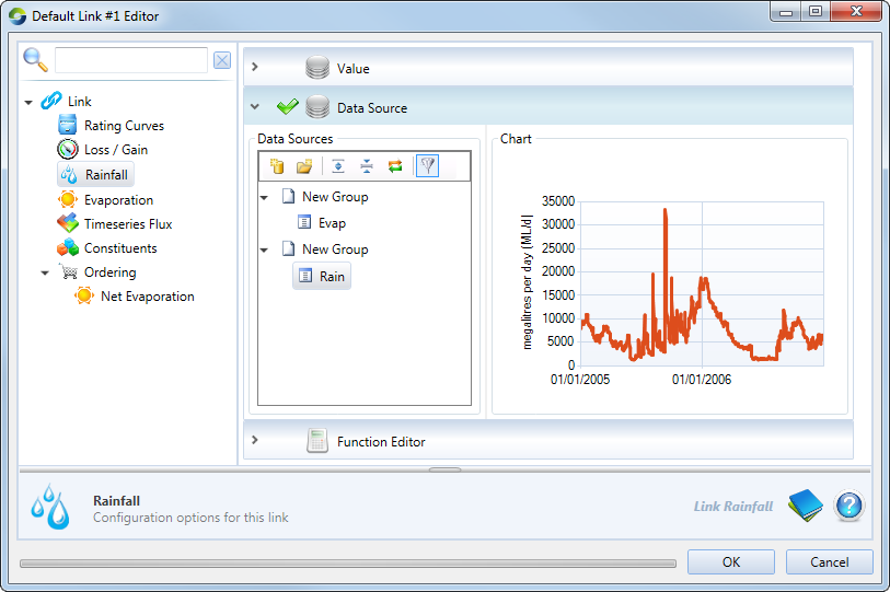
Rainfall on link surfaces
To specify the rate of precipitation per unit of surface area, choose Rainfall. Just like evaporation, this can be specified as a single value, as a time series (format shown in Table 5) or an expression. A time series can have multiple columns containing rainfall data.
Figure 11. Link (Storage routing, Rainfall)
Timeseries Flux
This allows the input of a time series of total water lost or gained on a link. Values can be positive or negative. A negative value denotes water returned to the link (a gain). See also Link losses and gains.
Figure 12. Link (Storage routing, Timeseries flux)
Constituents
Before you can configure constituents for a link, you must define them first for the scenario using Refer to Links.
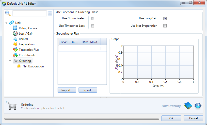
Ordering at links
Figure 13. Link (Ordering)
Ownership at links
Ownership must be enabled at the scenario-level (using Edit » Ownership) prior to configuring ownership at storage routing links. Refer to Ownership for details.