Note: This is documentation for version 4.11 of Source. For a different version of Source, select the relevant space by using the Spaces menu in the toolbar above
GR4J - SRG
The GR4J model is a catchment water balance model that relates runoff to rainfall and evapotranspiration using daily data. The model contains two stores and has four parameters.
Scale
GR4J operates at a catchment scale with a daily time-step.
Principal developer
The development of the GR4J model was initiated by Claude Michel at the beginning of the 1980s at Cemagref, a public research institute in France. The first version of the model only had a single parameter. Further development of the GR4J model was undertaken using a modelling approach where large numbers of catchments were used to evaluate and improve the model.
The GR4J modelling approach is mainly empirical (Michel et al., 2006), and consists of searching data for the most efficient model structures, with the objective of getting a general, efficient and robust model. The result being a parsimonious hydrological model, with successive improved versions. The main stages of the GR4J model development were:
- 3-parameter version proposed by Edijatno and Michel (1989) and Edijatno (1991). This provided the groundwork for further model development through testing and refinement;
- 4-parameter version proposed by Nascimento (1995) and detailed by Edijatno et al. (1999) (with one fixed parameter);
- 4-parameter version proposed by Perrin (2000) and detailed by Perrin (2002) and Perrin et al. (2003);
- 5-parameter version proposed by Le Moine (2008).
Scientific provenance
The successive versions of GR4J were widely tested on large sets of catchments in France but also in other countries, using demanding testing frameworks (Andréassian et al., 2009). The GR4J model has also been compared with other hydrological models and has provided comparatively good results (see eg Perrin et al., 2001; 2003; Vaze et al., 2011).
Version
Source v4.3
Dependencies
None.
Structure and processes
The mathematical details provided below follow the presentation of the model made by Perrin et al. (2003). Figure 1 shows a schematic diagram of the model.
Figure 1. Schematic diagram of the GR4J model
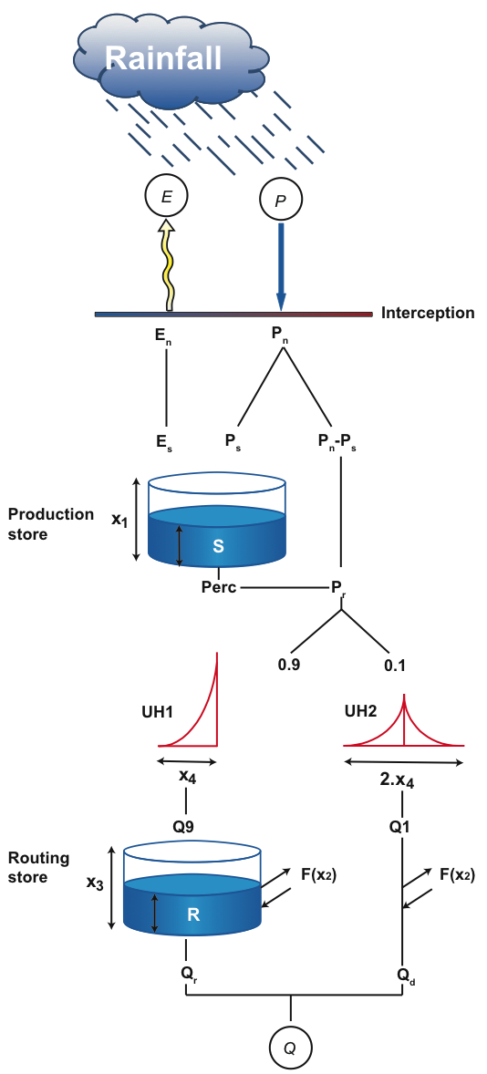
In the following, for calculations at a given time-step, we note P the rainfall depth and E the potential evapotranspiration estimate that are inputs to the model. P is an estimate of the areal catchment rainfall that can be computed by any interpolation method from available rain gauges. E can be based on long-term average monthly or daily values, which means the same potential evapotranspiration series could be repeated every year, although a recorded time series of E would be expected to give a better result.
All water quantities (input, output, internal variables) are expressed in mm, by dividing water volumes by catchment area, when necessary. All the operations described below are relative to a given time-step and correspond to a discrete model formulation (obtained after integration of the continuous formulation over the time-step).
Determination of net rainfall and PE
The first operation is the subtraction of E from P to determine either a net rainfall Pn or a net evapotranspiration capacity En. In GR4J, this operation is computed as if there were an interception storage of zero capacity. Pn and En are computed with the following equations:
| Equation 1 |  |
|---|
otherwise:
| Equation 2 |  |
|---|
Production store
This store can be considered as a soil moisture accounting (SMA) store. In case Pn is not zero, a part Ps of Pn fills the production store. It is determined as a function of the level S in the store by:
Equation 3 | 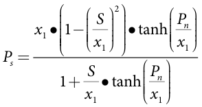 |
|---|
where the terms are defined in Table 1.
Table1. Model parameter definitions
| Parameter | Definition |
|---|---|
E | Potential areal evapotranspiration |
En | Net evapotranspiration capacity |
Es | Actual evaporation rate |
F(x2) | Groundwater exchange term |
P | Areal catchment rainfall |
Perc | Percolation leakage |
Pn | Net rainfall |
Pr | Total quantity of water to reach routing functions |
Pn-Ps | Amount of net rainfall that goes directly to the routing functions |
Ps | Amount of net rainfall that goes directly to the production store |
Q | Total stream flow |
Q1 | Output of UH2 |
Q9 | Output of UH1 |
Qd | Direct flow component |
Qr | Routed flow component |
R | Water content in the routing store |
S | Water content in the production store |
UH1, UH2 | Unit hydrographs |
x1 | Capacity of the production soil (SMA) store (mm) |
x2 | Water exchange coefficient (mm) |
x3 | Capacity of the routing store (mm) |
x4 | Time parameter (days) for unit hydrographs |
Equation 3 and Equation 4 result from the integration over the time-step of the differential equations that have a parabolic form with terms in (S/x1)², as detailed by (Edijatno and Michel, 1989).
In the other case, when En is not zero, an actual evaporation rate is determined as a function of the level in the production store to calculate the quantity Es of water that will evaporate from the store. It is obtained by:
Equation 4 | 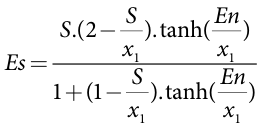 |
|---|
The water content in the production store is then updated with:
| Equation 5 |  |
|---|
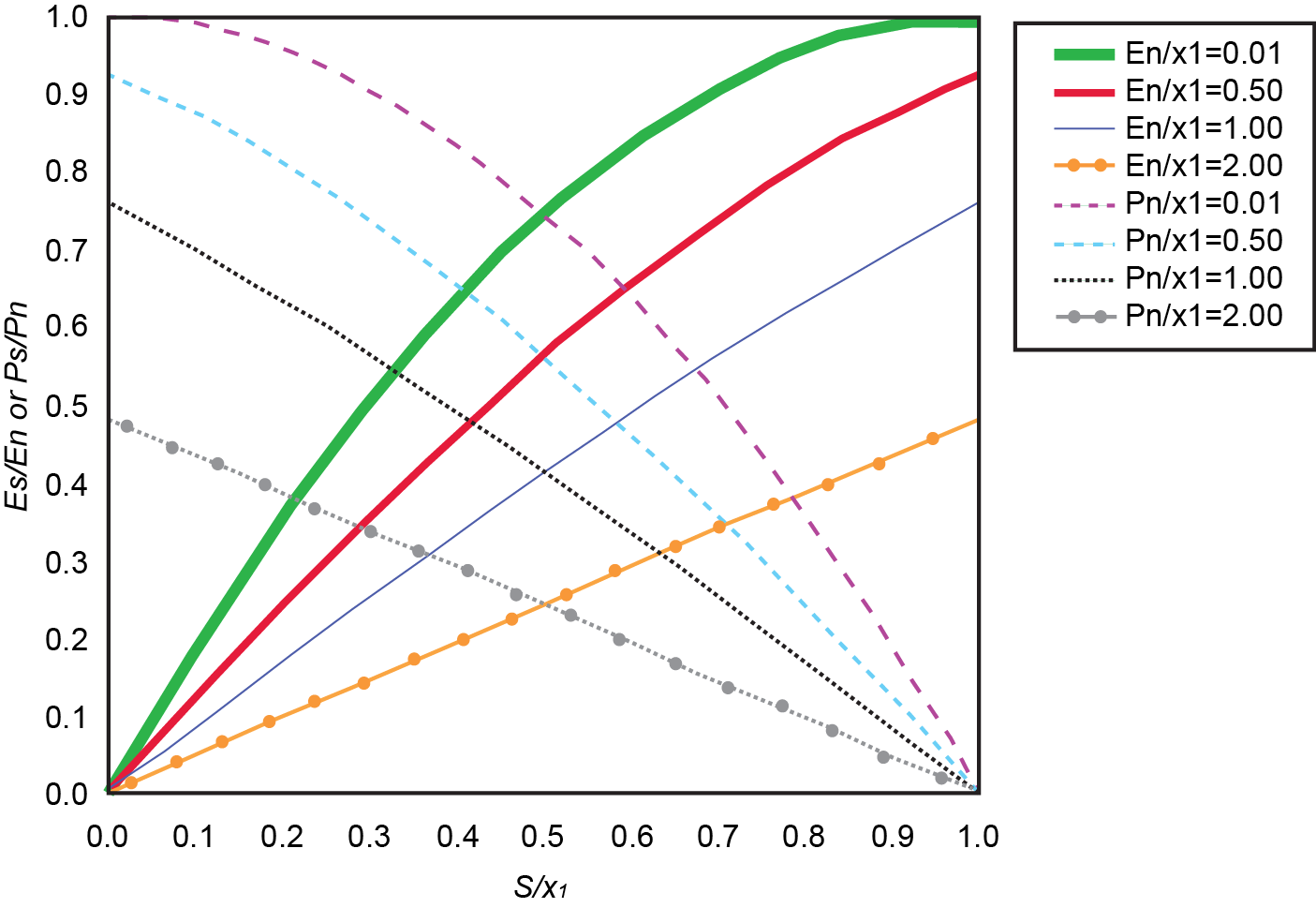
Note that S can never exceed x1. A representation of the rating curves obtained with Equation 3 and Equation 4 is shown in Figure 2.
Figure 2. Behaviour of the production functions (Es/En: solid line; Ps/Pn: dashed line) as a function of storage rate S/x1 for different values of En/x1 or Pn/x1
A percolation leakage Perc from the production store is then calculated as a power function of the reservoir content:
Equation 6 |  |
|---|
Perc is always lower than S. The reservoir content becomes:
| Equation 7 |  |
|---|
The percolation function in Equation 6 occurs as if it originated from a store with a maximum capacity of 9÷4•x1. Given the power law of the mathematical formulation, this means that the percolation does not contribute much to the stream flow and is interesting mainly for low flow simulation.
Linear routing with unit hygrographs
The total quantity Pr of water that reaches the routing functions is given by:
| Equation 8 |  |
|---|
Pr is divided into two flow components according to a fixed split: 90 % of Pr is routed by a unit hydrograph UH1 and then a non linear routing store, and the remaining 10% of Pr is routed by a single unit hydrograph UH2. With UH1 and UH2, one can simulate the time lag between the rainfall event and the resulting stream flow peak. Their ordinates are used in the model to spread effective rainfall over several successive time-steps. Both unit hydrographs depend on the same time parameter x4 expressed in days. However, UH1 has a time base of x4 days whereas UH2 has a time base of 2•x4 days. x4 can take real values and is greater than 0.5 days.
In their discrete form, unit hydrographs UH1 and UH2 have n and m ordinates respectively, where n and m are the smallest integers exceeding x4 and 2•x4 respectively. This means that the water is staggered into n unit hydrograph inputs for UH1 and m inputs for UH2. The ordinates of both unit hydrographs are derived from the corresponding S-curves (cumulative proportion of the input with time) denoted by SH1 and SH2 respectively. SH1 is defined along time t by:
| Equation 9 |  |
|---|
| Equation 10 |  |
|---|
| Equation 11 |  |
|---|
SH2 is similarly defined by:
| Equation 12 |  |
|---|
Equation 13 | 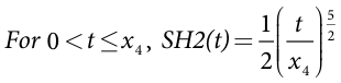 |
|---|
Equation 14 | 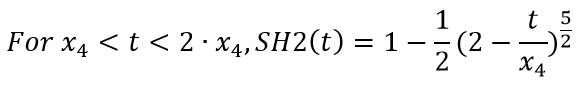 |
|---|
| Equation 15 |  |
|---|
UH1 and UH2 ordinates are then calculated by:
| Equation 16 | 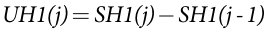 |
|---|
| Equation 17 |  |
|---|
where:
j is an integer.
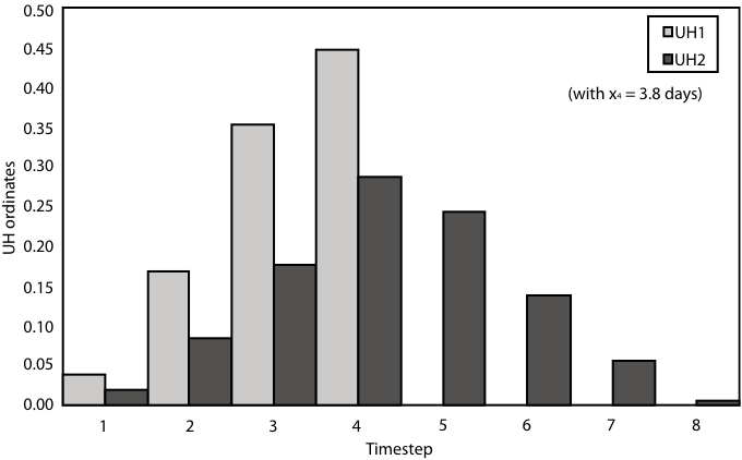
If 0.5 ≤ x4 ≤ 1, UH1 has a single ordinate equal to one and UH2 has only two ordinates. Figure 3 shows an example of unit hydrograph ordinates for x4 = 3.8 days.
Figure 3. Example of the ordinates of UH1 and UH2 for parameter x4 = 3.8 days
At each time-step, the outputs Q9 and Q1 of the two unit hydrographs correspond to the discrete convolution products and are given by:
Equation 18 |  |
|---|
Equation 19 |  |
|---|
where:
Equation 20 |  |
|---|
Inter catchment groundwater exchange
A groundwater exchange term F that acts on both flow components, is then calculated as:
Equation 21 |  |
|---|
Where R is the level in the routing store, x3 its "reference" capacity and x2 the water exchange coefficient. x2 can be either positive in case of water imports, negative for water exports or zero when there is no water exchange. The higher the level in the routing store, the larger the exchange. In absolute value, F cannot be greater than x2: x2 represents the maximum quantity of water that can be added (or released) to (from) each model flow component when the routing store level equals x3. Note that Le Moine (2008) proposed an improved formulation of this function, with an additional parameter.
Non linear routing store
The level in the routing store is updated by adding the output Q9 of UH1 and F as follows:
| Equation 22 |  |
|---|
The outflow Qr of the reservoir is then calculated as:
Equation 23 |  |
|---|
Qr is always lower than R, as shown in Figure 4. The formulation of the output of the store is the same as the percolation from the SMA store. The level in the reservoir becomes:
| Equation 24 |  |
|---|
Note that, although the reservoir can receive a water input greater than the saturation deficit x3-R at the beginning of a time-step, the level in the reservoir can never exceed the capacity x3 at the end of a time-step, as shown in Figure 4. Therefore, the capacity x3 could be called the "one day ahead maximum capacity". This routing store is able to simulate long stream flow recessions, when necessary.
Figure 4. Illustration of the outflow Qr from the routing reservoir as a function of the level in the store after the introduction of input Q9
Total stream flow
Like the content of the routing store, the output Q1 of UH2 is subject to the same water exchange F to give the flow component Qd as follows:
| Equation 25 |  |
|---|
Total stream flow Q is finally obtained by:
| Equation 26 |  |
|---|
The Source implementation of GR4J includes a baseflow filter than can be used to estimate a baseflow amount from the overall runoff flux, Q. GR4J uses the same baseflow filter as is used in the observed catchment runoff depth model (see the Observed catchment runoff depth - SRG page for more information).
Input data
The model requires daily rainfall and potential evapotranspiration data. The rainfall and evaporation data sets need to be continuous and overlapping.
Parameters or settings
Information on parameters is provided in Table 2. All four parameters are real numbers. x1 and x3 are positive, x4 is greater than 0.5 and x2 can be either positive zero or negative.
Table 2: Parameters in GR4J and their default values
Parameter | Description | Units | Default | Range |
x1 | Capacity of the production soil (SMA) store | mm | 350 | 1-1500 |
x2 | Water exchange coefficient | none | 0 | -10.0-5.0 |
x3 | Capacity of the routing store | mm | 40 | 1-500 |
x4 | Time parameter for unit hydrographs | days | 0.5 | 0.5-4.0 |
k | Filter parameter given by the recession constant (as in observed catchment runoff depth model) Note: not the same k as used in equations 18 and 19, above. | none | n.a. | 0-1 |
C | Shape parameter (as in observed catchment runoff depth model) | none | n.a. | 0-1 |
Note that some coefficients in the model equations above appear as fixed values, eg. a power 4 in Equation 6 and Equation 20, a fixed split 10% - 90% of effective rainfall, a 2.5 exponent in the computation of the unit hydrographs, a 2.25 coefficient related to the percolation function in Equation 6. These values were chosen as those yielding the best model results in many different test conditions. They were fixed because leaving them free did not significantly improve (or even degraded) the model results while adding unhelpful complexity to the model structure.
Most optimisation algorithms used to calibrate the model parameter values require knowledge of an initial parameter set. This initial set may consist of median values obtained on a large variety of catchments (for example, see Table 3). Approximate 80 % confidence intervals for the four parameters are also provided in Table 3. They were derived from the 0.1 and 0.9 percentiles of the distributions of model parameter values obtained over a large sample of catchments. Given the small number of model parameters, simple optimisation algorithms are generally capable of identifying parameter values yielding satisfactory results. The choice of an objective function depends on the objectives of model user. Note that care should be taken to set appropriate initial conditions of the internal state variables in the model to avoid discrepancies at the beginning of the simulation periods. One year can be used for model warm-up at the beginning of each simulation.
Table 3: Values of median model parameters and approximate 80% confidence intervals
| Parameter | Median Value | 80% Confidence Interval |
|---|---|---|
x1 | 350 | 100-1200 |
x2 | 0 | -5 to 3 |
x3 | 90 | 20-300 |
x4 | 1.7 | 1.1-2.9 |
Leaving both the k and C parameters at 0 has the effect of disabling the baseflow filter, and all runoff will be reported as quickflow.
Output data
The model outputs daily surface flow and intercatchment groundwater exchange flow, expressed in mm/day.
The Source implementation of GR4J includes a baseflow filter component. This does not change the overall results of GR4J, but does introduce slow flow and quick flow as additional outputs, which can be useful in some circumstances. For example, the baseflow filter provides a means to use GR4J with the EMC/DWC constituent generation model. This baseflow filter is optional and there will be no effect on any results if the filter parameters (k and C) are both left at their default values of 0. Use of this filter is described in the section on observed runoff, and also Hydrological Recipes, Estimation Techniques in Australian Hydrology, R. B. Grayson et al. 1996, Cooperative Research Centre for Catchment Hydrology, which can be downloaded at:
http://www.ewater.com.au/uploads/files/Grayson-1996-Hydrological-Recipes-CRCCH.pdf
References
Grayson, R. B., Argent, R., M., Nathan, R., J., McMahon, T., A., Mein, R. G. (1996), Hydrological Recipes, Estimation Techniques in Australian Hydrology, Cooperative Research Centre for Catchment Hydrology.
Perrin, C., C. Michel, and V. Andréassian (2003), Improvement of a parsimonious model for streamflow simulation, J. Hydrol., 279, 275-289.
Bibliography
Andréassian, V., C. Perrin, L. Berthet, N. Le Moine, J. Lerat, C. Loumagne, L. Oudin, T. Mathevet, M. H. Ramos, and A. Valéry (2009), Crash tests for a standardized evaluation of hydrological models, Hydrol. Earth. Syst. Sci., 13, 1757-1764.
Edijatno (1991), Mise au point d’un modèle élémentaire pluie-débit au pas de temps journalier, Thèse de Doctorat thesis, 242 pp, Université Louis Pasteur/ENGEES, Strasbourg.
Edijatno, and C. Michel (1989), Un modèle pluie-débit journalier à trois paramètres, La Houille Blanche, 113-121.
Edijatno, N. O. Nascimento, X. Yang, Z. Makhlouf, and C. Michel (1999), GR3J: a daily watershed model with three free parameters, Hydrol. Sci. J., 44, 263-277.
Le Moine, N. (2008), Le bassin versant de surface vu par le souterrain : une voie d’amélioration des performances et du réalisme des modèles pluie-débit ?, Thèse de Doctorat thesis, 324 pp, Université Pierre et Marie Curie, Paris.
Michel, C., Perrin, C., Andréassian, V., Oudin, L. and Mathevet, T.(2006) Has basin-scale modelling advanced beyond empiricism? In: Andréassian, V., Hall, A., Chahinian, N. and Schaake, J. (eds) Large sample basin experiments for hydrological model parameterization: results of the model parameter experiment (MOPEX) 2006 pp. 108-116. IAHS Publication 307.
Nascimento, N. O. (1995), Appréciation à l’aide d’un modèle empirique des effets d’action anthropiques sur la relation pluie-débit à l’échelle du bassin versant, Thèse de Doctorat thesis, 550 pp, CERGRENE/ENPC, Paris.
Perrin, C. (2000), Vers une amélioration d’un modèle global pluie-débit au travers d’une approche comparative, Thèse de Doctorat thesis, 530 pp, INPG (Grenoble) / Cemagref (Antony).
Perrin, C. (2002), Vers une amélioration d’un modèle global pluie-débit au travers d’une approche comparative, La Houille Blanche, 84-91.
Perrin, C., C. Michel, and V. Andréassian (2001), Does a large number of parameters enhance model performance? Comparative assessment of common catchment model structures on 429 catchments, J. Hydrol., 242(3-4), 275-301.
Vaze, J., Chiew, F. H. S., Perraud, JM., Viney, N., Post, D. A., Teng, J., Wang, B., Lerat, J., Goswami, M., 2011. Rainfall-runoff modelling across southeast Australia: datasets, models and results. Australian Journal of Water Resources, Vol 14, No 2, pp. 101-116.