Note: This is documentation for version 4.11 of Source. For a different version of Source, select the relevant space by using the Spaces menu in the toolbar above
IQQM Crop Model SRG
Source models the use of water by a combination of supply point and water user nodes. The water user node provides a range of demand models that include the IQQM crop model. The IQQM crop model operates on a daily basis generating demands and extracting water to meet these demands via the water user and supply nodes. The model can be applied in both regulated and unregulated systems.
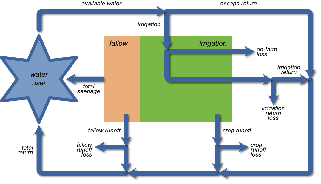
The IQQM crop model maintains a soil moisture store for each irrigated crop as well as the fallow land with the combined areas of these stores equal to the maximum irrigable area multiplied by a development factor. The fluxes associated with the crop stores are effective rainfall, irrigation, runoff, evapotranspiration and seepage. The fluxes associated with the upper fallow store are rainfall, runoff, evaporation and infiltration and with the lower fallow store are infiltration and seepage. Irrigation water is supplied by the water user and total return flow and seepage are returned to the water user. The fate of the return flow and seepage is dependent on how the water user is configured to manage this water. Return flow can be sent to the water user storage or returned to a confluence node. Seepage can be input to a surface water ground water interaction model. Alternatively these fluxes can be treated as a loss.storage or returned to a confluence node. Seepage can be input to a surface water ground water interaction model. Alternatively these fluxes can be treated as a loss.
| Equation 1 | 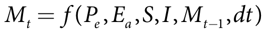 |
where:
Mt is the soil moisture depth at the end of the current time-step (m)
Mt-1 is the soil moisture depth at the end of the previous time-step (m)
Pe is the effective rainfall (m/s)
Ea is the actual evapotranspiration (m/s)
S is the seepage (m/s)
I is the irrigation applied per unit area (m)
dt is the model time-step (s)
The IQQM crop model has two planting decision dates each year. These are for the primary and secondary crops. Primary crops are the crops that are predominantly supplied by irrigation. In the Murray-Darling basin this is usually summer crops. The secondary crops are largely rain fed and use any remaining irrigation to maintain soil moisture. In the Murray-Darling Basin these are usually winter crops.
On a decision date the user can optionally specify a farmer’s risk function that decides on the area of primary or secondary crops to plant. The function takes into consideration available resource, expected resource and antecedent conditions to determine the area to plant. Note that only a decision on area is made at the planting decision date and the crop area only becomes active on the specified crop start date.
Perennial crops such as orchards and trees grow all year and are considered as primary crops in the model. The area of these crops will change on the planting decision date.
Scale
IQQM crop model is applied at a point scale and operates on a daily time-step.
Principal developer
NSW Office of Water
Scientific provenance
The IQQM crop model is based on a crop model developed by Lyall & Macoun Consulting Engineers (1986) for the WARAS Lachlan daily model. The model has been substantially modified by the former NSW Department of Land and Water Conservation to accommodate the different irrigation conditions in other NSW regions and internationally (DIPNR, 2004). The IQQM Fortran code was rewritten to fit within the water user structure of Source in C# by New South Wales Office of Water and eWater.
The crop factors used to determine actual evapotranspiration are based on the FAO56 (Allen, et al, 1998) approach. For further information on how this approach is implemented in Source see the Irrigation Demand Model Crop Factors SRG entry. Source also offers sufficient flexibility to apply daily crop factors if they are known for a particular crop based on a different source or method.
Version
Source V3.02
Dependencies
The IQQM Crop Model is applied through a water user node, which must be connected to at least one supply point node to provide water to satisfy the irrigation demand.
Availability/conditions
Automatically included with Source.
Structure and processes
The IQQM Crop Model is a daily soil moisture accounting demand model available for use within a Water User node. It generates water requirements for irrigated crops. Crop water requirements are used to generate demands in regulated and unregulated systems, orders and opportunistic requests within regulated systems and to extract water from a water source, subject to water availability and extraction constraints. Note orders are supplied from storages while request are allocated at off allocation nodes. Water is extracted from an optional water user storage and at Supply Point nodes and is directed to the associated water user node to be distributed to the demand model as a first priority.
The schematic of the irrigable area is shown in Figure 1 and the conceptualisation of the farm supply system is shown in Figure 2. A description of the parameters used by the model is in the Importing data section of the User Guide.
Figure 1. Schematic of irrigable area
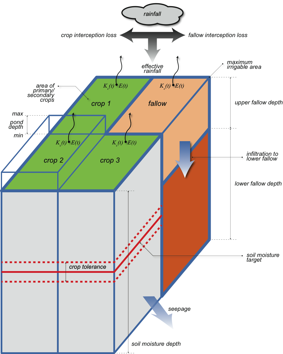
Figure 2. Conceptualisation of the farm supply system assumptions and constraints
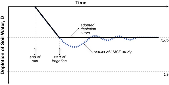
In developing the original crop model, Lyall & Macoun Consulting Engineers (1986) conducted some numerical tests on 1000 conceptual farms with random distributions of soil moisture and evapotranspiration. During these tests it was assumed that each farm was irrigated when the soil moisture reached zero ie. fully depleted. The study found that irrigation recommenced some time after rainfall and that the depletion curve followed a damped oscillating pattern around half the soil moisture capacity. This is shown (typically) in Figure 3 for a period following saturating rain. For simplicity of modelling, the oscillating curve is replaced by two straight lines as shown in Figure 5.
Figure 3. Irrigation scheduling and adopted soil moisture target curve (a)
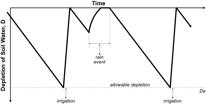
Figure 4. Irrigation scheduling and adopted soil moisture target curve (b)

Figure 5. Irrigation scheduling and adopted soil moisture target curve (c)
Theory
The following covers aspects of the theory relevant to IQQM crop model including:
- Area planting decision
- Irrigation demand and opportunistic requirements
- Irrigation application
The workflow between the IQQM crop model and the Water User for each model time-step is as follows:
- When the first supply node is reached in the ordering phase the IQQM crop model checks if it is a planting decision date. If so IQQM determines the area of crops to plant for the respective decision date.
- The IQQM crop model determines if it is the start date for a crop. If so it allocates a soil moisture store from the fallow area based on the area decided on the planting date for the season associated with the crop.
- Based on the soil moisture state for each crop the IQQM crop model calculates today’s and forecast demands and opportunistic requirements (normally these are the same number) up to the maximum delivery time of supply storages and off allocation nodes respectively. Note in unregulated systems this is just today’s requirement. This is subsequently passed to the water user node.
- The water user node allocates the calculated demands and opportunistic requirements to supply points and the optional water user storage subject to supply limitations and licences in regulated systems.
- When the first supply point node (noting that a water user node can be connected to multiple supply point nodes) is reached in the flow phase the water user gathers all of the available water from all supply points and the optional water user storage subject to today’s demand and opportunistic requirement determined in the third step.
- The IQQM crop model applies the available water to the crops.
- The IQQM crop model then determines and passes back any seepage and return flow to the water user node.
- If the water user node is connected to a groundwater model then the seepage is input into the groundwater model.
- If the water user node has a storage then a proportion of the return water is put into the storage. Separate return proportions can be specified for water generated from rainfall derived runoff and irrigation applications.
- If the water user node is connected to a return confluence any remaining return water or spills from the water user storage are passed to the confluence node.
Forecast irrigation demands and opportunistic requirements are estimated up to the maximum delivery time from the furthest accessible storage and the delivery time from the furthest of the next upstream off allocation sharing nodes respectively. The forecast demand is based on an estimate of the volume required to maintain the soil moisture at a target state or minimum pond depth (for ponded crops such as rice) assuming no rainfall and a forecast evaporation rate. In most cases the opportunistic requirement is equal to the demand. In cases where a crop tolerance is specified (further discussed in a later section on Projected demands and requirements) the opportunistic requirement will be assumed to meet the soil moisture target plus the crop tolerance. Note opportunistic requirements are met from overbank flows and off allocation sharing where specified.
Area planting decision
The area to be planted by the IQQM crop model may be fixed or optionally determined at the start of a primary or secondary irrigation season based on a farmer’s risk function. The area to plant is determined at the user defined decision date for the primary and secondary irrigation seasons. In the IQQM crop model, farmer’s risk can be modelled in two different ways; an area based approach and a volume based approach. An overview of these follows and they are described in more detail in separate sections on the Area Method and the Volume Method below.
The area based approach is based on a direct conversion rate (in ML/ha) from the farmer’s available resources to the planted area. The farmer’s available resources comprise water in the water user storage and any water available in account balances. The risk is influenced by the slope of the risk line relative to the actual water requirement of the crop. For example if a cotton crop requires 8 ML/ha and the slope is 6 ML/ha then the farmer is taking risk on the remainder of the water becoming available post decision. This approach can be applied in both regulated and unregulated systems.
The volume based approach uses the risk function to calculate the expected available water resource during the season. Based on the model’s calculation of crop requirements and the expected rainfall in the growing season, the expected available resource is then converted into an area to plant. This approach is relevant for regulated river systems that have allocation systems. It is based on the assumption that there will be an increase in allocation during the season. The increase effectively allows for additional inflows to the supply reservoirs that are expected to become available during the season.
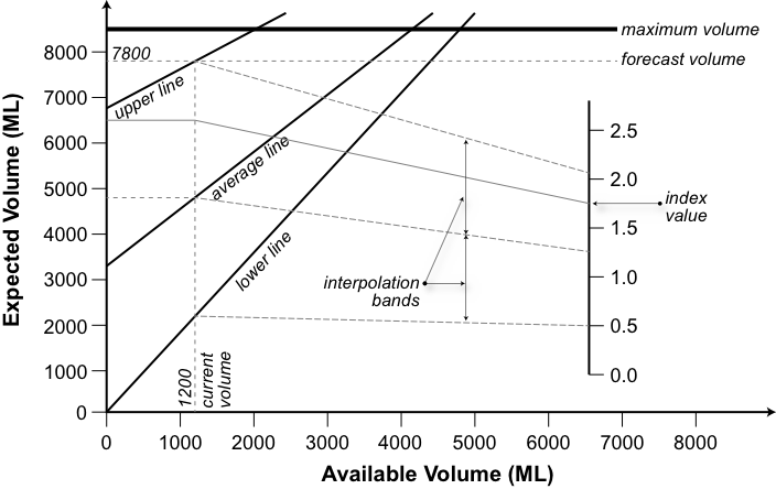
For both of these types of risk functions, the value of the risk function depends on the antecedent climatic conditions. For example, in a wet year, the farmers may take more risk to recognise the higher probability of improved resources throughout the year. The modeller can define risk functions for dry, average and wet conditions. The final function used by Source is based on an interpolation between these curves based on current antecedent conditions. The index for antecedent conditions is calculated as follows;
- the ratio of the six monthly sum of a time series data (typically inflows) to the median prior 6-monthly inflows for the volume based function (Figure 6), and
- 2 x the ratio of the fallow soil moisture to the fallow soil moisture capacity the day before the planting decision date for the area based function.
Figure 6. Volume based farmer’s risk function
If there is more than one crop type within a season, the area to be planted is divided between the crops based on the user defined proportion values. Although the planting decision is made on a particular date the crop area does not become allocated until the start date for that particular crop.
Risk function - Area method
The area to be planted is determined based on:
- available water resources, which is the water available in the water user storage plus the sum of all the account balances;
- an index of antecedent conditions using fallow soil moisture for the day before the planting decision date; and
- a relationship between available water and crop area with different relationships applying to wet, average and dry conditions. The index is used to determine the final relationship used.
The user defined risk function parameters are used in the following calculation:
| Equation 2 | 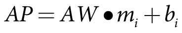 |
where:
AP is the area to plant in the irrigation season (m2)
AW is the available resource (m3)
mi is the slope of index curve for the irrigation season (m-1)
bi is the intercept of index curve for the irrigation season (m2)
i is the curve identifier
The calculation in Equation 2 may be constrained based on maximum seasonal planting areas and also based on minimum and maximum parameters in the risk function (refer to Limits to Area Planted).
The slope and intercept of the farmers risk function can be derived by plotting historic data on available resources for each water year versus the area planted for the irrigation season (separate functions can be derived for wet, dry and average conditions if required and data availability permits) This method does not take into consideration other factors that may affect planting decisions such as changes in water sharing rules, water use accounting rules and external factors such as terms of trade/ commodity prices. If scenarios are to be modelled which entail a change in any of these factors, then the function should be re-derived.
If the modeller wants to define the risk function so that some of the water user’s account balance is reserved for the secondary crop then this can only be achieved indirectly by defining a function which plants less area given an available resource. For example if x ML needs to be reserved for the secondary crops then xslope should be subtracted from the intercept for each of the curves for the primary crop. Logically the intercept should not be less than zero.
The choice of slope and intercept values to use depends on the current index value which evaluates how wet, average or dry the conditions are using fallow soil moisture calculated at the end of the previous time-step (ie. the day before the planting decision date):
| Equation 3 | 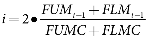 |
|---|
where:
i is the index used to interpolate between risk curves
FUMt-1 is the fallow upper soil moisture at the end of the previous time-step (m)
FLMt-1 is the fallow lower soil moisture at the end of the previous time-step (m)
FUMC is the fallow upper soil moisture capacity (m)
FLMC is the fallow lower soil moisture capacity (m)
If the calculated index ratio falls between two specified curve index values, the area will be calculated based on interpolation between those index results (Equation 4) The lower line and the upper line sets the limits of the area to be irrigated ie. values are not extrapolated. For example, if the index value is greater than the wet relationship index value then the wet index slope and intercept is used.
Equation 4 | 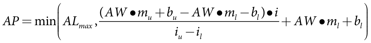 |
where:
AP is the area to plant in the irrigation season (m2)
AW is the available resource (m3)
i is calculated in Equation 3
mu is the slope of the upper curve iu for the irrigation season(m-1)
bu is the intercept of the upper curve iu for the irrigation season (m2)
iu is the index of the upper curve for the irrigation season
ml is the slope of the lower curve iu for the irrigation season (m-1)
bl is the intercept of the lower curve iu for the irrigation season (m2)
il is the index of the lower curve for the irrigation season
ALmax the specified maximum area for the growing season (m2)
Risk function - Volume method
The area planted is determined based on:
- a user defined risk function which calculates the expected available water resources based on the current available water resource;
- an index of antecedent conditions based on the user-specified inflow data;
- model calculated average total crop water requirements for a irrigation season; and
- expected usable rainfall in the irrigation season.
The user defined risk function parameters are used in the following calculation (see Figure 6):
| Equation 5 | 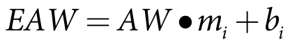 |
where:
EAW is the expected available resource (m3)
AW is the available resource (m3)
mi is the slope of the index curve i for the irrigation season
bi is the intercept of the index curve i for the irrigation season (m3)
i is the curve identifier
The planted area is then calculated based on the expected available resource, the estimated crop water requirement and the expected rainfall in the growing season, it is constrained by maximum area limits for the farm and the season.
Equation 6 | 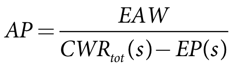 |
where:
AP is the area to plant in the irrigation season s (m2)
EAW is the expected available resource (m3)
CWRtot(s) is the total crop water depth (m) requirement for the planted area decision season s (m)
EP(s) is the expected precipitation depth in the planted area decision season s (m)
s is the planted area decision season
Equation 6 demonstrates that the model calculates the crop demand in this risk method based on the average crop evapotranspiration with specified allowance for the minimum or expected rainfall that will occur during the growing season. If the user defines a daily pattern of average evaporation then this is used otherwise a daily pattern is generated based on the input evaporation data.
The total crop water depth requirements are determined during model initialisation using the following formula:
Equation 7 | 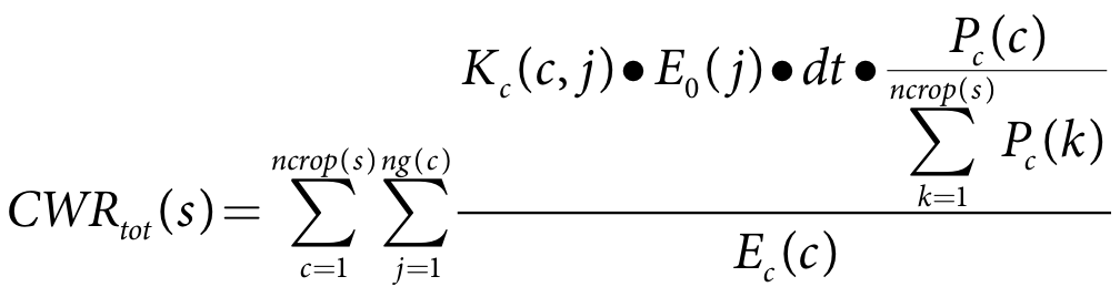 |
where:
CWRtot(s) is the total crop water requirement for season s (m)
ncrop(s) is the number of crops in season s
ng(c) is the number of growing days for crop c
Kc(c,j) is the crop factor for crop c on day j
E0(j) is the forecast potential evapotranspiration rate on day j (m/s)
dt is the model time-step (s)
Pc(c) is the proportion of area of crop c
Ec(c) is the irrigation efficiency of crop c
s is the planted area decision season
The choice of slope and intercept values to use depends on the current index value which evaluates how wet, average or dry the conditions are (see Figure 6) The volume based risk function uses inflow index based on the supplied time series data:
| Equation 8 | 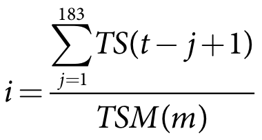 |
| Equation 9 |
|
where:
i is the index used to interpolate between risk curves
TS(t-j+1) is the time series inflow at time t-j+1 (m3/s)
TSM(m) is the specified median of the previous 183 days of inflow for all years in the time series
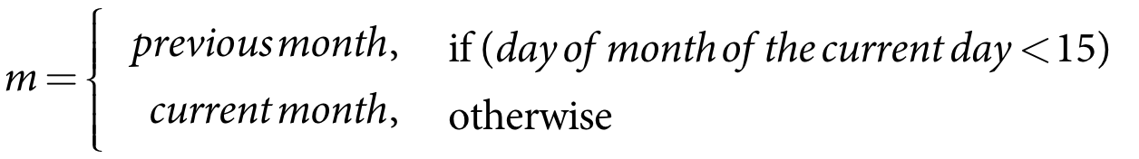
m is the index month
If the calculated index ratio falls in between the two specified index values, the expected volume will be calculated based on interpolation between those index results (Equation 4) The lower line and the upper line set the limits of the expected volume ie. the values are not extrapolated. For example, if the index value is greater than the wet relationship index value then the wet index slope and intercept are used.
Limits to Area Planted
The total area planted within a water year is limited by the following:
- Total crop area is limited to the Maximum Irrigable Area (IAmax=Atotdf) which is the total area of the farm multiplied by the development factor.
- Maximum planting area in the respective primary or secondary season. Note neither of these should exceed the maximum irrigable area (Amax(s)=min(IAmax,Amax(s))).
- For the volume method a minimum area is specified (Equation 11)
- For the area method the risk function can be limited by two minimum areas.
- A user-specified area threshold to make a decision to plant or not in the current irrigation season. If the calculated area is less than this threshold, then there is no area to be planted (Equation 212).
- Minimum area to plant based on the risk function. If the calculated area is less than this value and the index is above the average value, then plant this area (ie. this can be used to simulate farmers taking more risk in this situation) This parameter only applies when using the area based risk function.
| Equation 10 |  |
Volume based
| Equation 11 |  |
Area based
| Equation 12 | 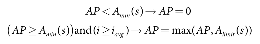 |
where:
AP is the area to plant in the irrigation season (m2)
Amax(s) is maximum planted area for season s (m2)
i is the index used to interpolate between risk curves
iavg is the index value of the average risk curve
Volume based
Amin(s) is the user-specified minimum area to plant for season s (m2)
Area based
Amin(s) is the user-specified minimum area threshold to plant crops for season s (m2)
Alimit(s) is the user-specified minimum area to plant for season s (m2)
Irrigation demand and opportunistic requirements
The irrigation demand and opportunistic requirements are determined each day and for regulated systems they are predicted for a defined time into the future. In projecting the soil moisture conditions the model takes into consideration evapotranspiration, seepage and water that has been previously ordered. A demand for irrigation is generated when the projected soil moisture level is less than the target soil moisture level. Orders are generated to satisfy this irrigation demand with consideration given to delivery time from the regulated water source to the extraction node.
The calculation of the irrigation demand requires a calculation of the estimated crop evapotranspiration and subsequently the estimated soil moisture shortfall. The following two sections provide some background on these components of the model.
Crop evapotranspiration (Ec)
Crop evapotranspiration is determined by multiplying potential reference crop evapotranspiration by a crop factor (Kc) The potential evapotranspiration is a time series input that may be calculated directly by the Penman-Monteith or equivalent method. Alternatively pan evaporation data may be modified by a pan factor (Kpan) to convert to potential reference crop evapotranspiration.
The method for defining crop factors is based on FAO56 (Allen, et al, 1998), which represents the growth period of each crop by four developmental stages defined as curves. The four stages are:
initial stage
also called the "establishment stage", this stage occurs between planting and when there is approximately 10% ground cover. Water requirements are low and constant.
crop development stage
also called the "vegetative stage", this stage has a rapid increase in the amount of water required by the crop until there is generally about 70%-80% ground cover and maximum rooting depth is achieved.
mid-season stage
also called the "flowering stage", this stage requires the maximum amount of water in the life of the crop.
late stage
also called the "yield" and/or "ripening stage", the water requirement is for crop ripening and reaching maturity.
Crop factors for each modelled time-step are interpolated using co-ordinates of the curve or alternatively entered as a daily pattern. Note crop factors are entered based on growing days and are offset by the start date of the crop.
Setting the crop area and soil moisture
IQQM Crop Model has individual single layer soil moisture stores for each crop type. The irrigation period starts at the specified crop start date when the crop factor becomes greater than zero. The area planted is based on the planting decisions for the associated season and a user-specified proportion (Equation 13) The fallow area is debited for the area of the crop planted (Equation 14). When the crop is planted the initial soil moisture is equal to the total soil moisture for the fallow (Equation 15).
Equation 13 | 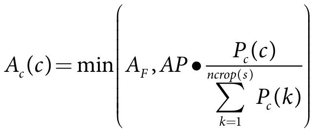 |
| Equation 14 |  |
| Equation 15 |  |
where:
AP is the area to plant in the irrigation season (m2)
AF is the current fallow area (m2)
Ac(c) is the area of crop c to be planted in the current season (m2)
ncrop(s) is the number of crops in irrigation season s
Pc(c) is the proportion of area of crop c
Mt(c) is the initial soil moisture for crop c (m)
FUMt-1 is the fallow upper soil moisture at the end of the previous time-step (m)
FLMt-1 is the fallow lower soil moisture at the end of the previous time-step (m)
When the crop has finished growing, which is identified when the crop factor becomes zero, then the crop area (Equation 13) and moisture is transferred back to fallow (Equation 16 and Equation 17).
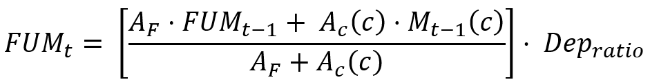
| Equation 16 |
|
| Equation 17 |
|

| Equation 18 |
|
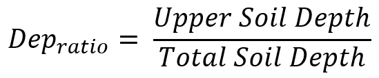
Depratio is the proportion of Upper Soil in the soil profile under Fallow
| Equation 19 |
|
where:
FUMt is the fallow upper soil moisture at the end of the current time-step (m)
FLMt is the fallow lower soil moisture at the end of the current time-step (m)
FUMt-1 is the fallow upper soil moisture at the end of the previous time-step (m)
FLMt-1 is the fallow lower soil moisture at the end of the previous time-step (m)
Mt-1(c) is crop c soil moisture at the end of the previous time-step (m)
Ac(c) is the area of crop c (m2)
AF is the fallow area (m2)
Projected demands and requirements
The crop soil moisture is depleted by evapotranspiration and seepage and is replenished by rainfall and irrigation application. The objective of irrigation watering is to maintain the soil moisture at a target state. The target state may be fixed at half the soil moisture capacity, specified in a soil moisture target curve or for ponded crops (eg. rice) a minimum pond level can be specified. Optionally a crop tolerance (see Figure 1) can be specified as well as the target moisture state. In regulated systems, orders are placed when the soil moisture content is below the target moisture state less the crop tolerance, with the aim of bringing the soil moisture up to the target state plus crop tolerance. When meeting opportunistic requirements in regulated or unregulated systems, the aim is also to bring the soil moisture up to the target state plus crop tolerance.
The process for estimating the future demand (Itotdem) and opportunistic requirement (Itotreq) is:
- Calculate the crop water requirement - Equation 20
- Calculate the soil moisture level - Equation 21
- If ponded, adjust the soil moisture level - Equation 22
- Calculate the moist target minimum - Equation 23
- Calculate the moist target maximum - Equation 24
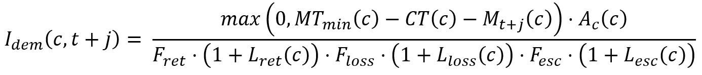
- Calculate the demand - Equation 25
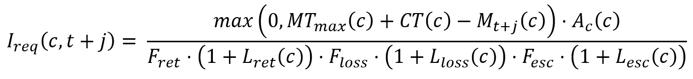
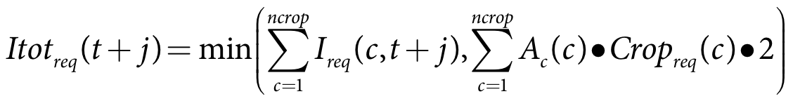
- Calculate the opportunistic requirement - Equation 26 through Equation 28
| Equation 20 |
|
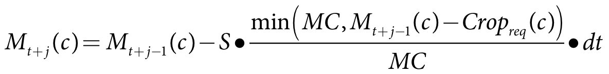
| Equation 21 |
|
| Equation 22 |
|

Equation 23 |
|

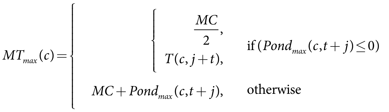
Equation 24 |
|
| Equation 25 |
|
| Equation 26 |
|
| Equation 27 | 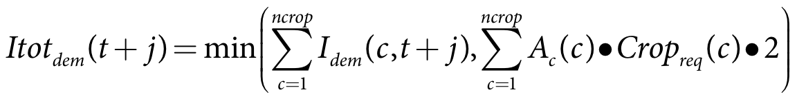 |
| Equation 28 |
|
|---|
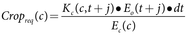
| Equation 29 | 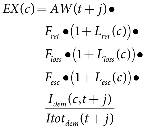 |
Irrigate
| Equation 30 | 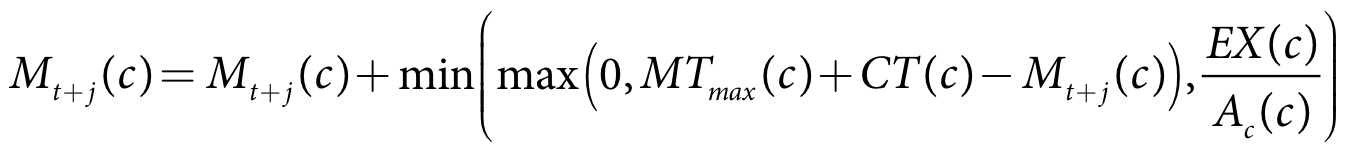 |
where:
Cropreq(c) is the depth requirement of crop c on day t+j (m)
Mt+j(c) is crop c soil moisture on day t+j (m)
Kc(c,t+j) is the crop factor for crop c on day t+j
E0(t+j) is the forecast potential evapotranspiration rate on day t+j (m/s)
Ec(c) is the irrigation efficiency of crop c
S is the seepage (m/s)
dt is the model time-step (s)
MC is the soil moisture capacity (m)
Pondmin(c,t+j) is the minimum pond depth on day t+j (m)
MTmin(c) is the minimum soil moisture target for crop c (m)
MTmax(c) is the maximum soil moisture target for crop c (m)
CT(c) is the crop tolerance for crop c (m)
T(c,t+j) is the soil moisture target (when specified) on day t+j (m)
Idem(c,t+j) is the demand for crop c on day t+j (m)
Ireq(c,t+j) is the opportunistic requirement for crop c on day t+j (m)
Ac(c) is the area of crop c (m2)
Lret(c) is the return loss for crop c
Fret(c) is the return loss factor
Lloss(c) is the on-farm loss for crop c
Floss(c) is the on-farm loss factor
Lesc(c) is the escape loss for crop c
Fesc is the escape loss factor
Itotdem(t+j) is the total demand on day t+j (m)
Itotreq(t+j) is the total opportunistic requirement on day t+j (m)
EX(c) is the irrigation water that is available for crop c on day t+j (m)
AW(t+j) is the available water on day t+j (m)
The required volume to maintain the soil moisture at target depletion level is limited to twice the total daily crop evapotranspiration requirement of all irrigated crop types.
The irrigation requirement of the crop may be less than the volume that needs to be extracted as there may be losses between the point of extraction and the point of irrigation. There are three such processes represented in the IQQM crop model as illustrated in Figure 2; on-farm loss, on-farm escape and irrigation returns. The on-farm escape and irrigation return can be returned to either the water user storage or the river.
Irrigation application
Each of the crop soil moisture stores is firstly updated for rainfall, evapotranspiration and seepage. Where the rainfall exceeds pond or soil moisture levels all or a portion of the rainfall will appear as runoff.
The rainfall reaching the soil moisture is the rainfall less rainfall interception loss and less evapotranspiration and is limited to the remaining soil moisture capacity plus 20% of the moisture capacity of the soil (Lyall & Macoun Consulting Engineers, 1986) It is evaluated using Equation 31 for soil effective rainfall:
Equation 31 | 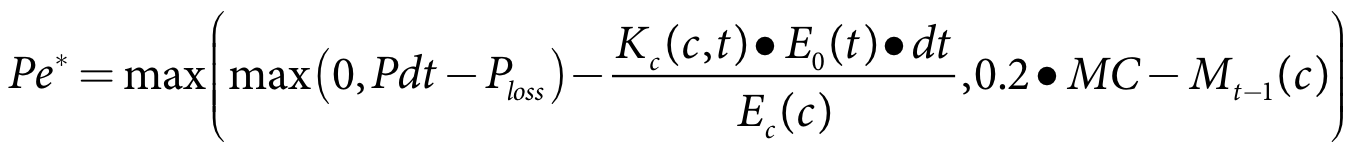 |
where:
Pe* is the soil rainfall depth for crop c on the current time-step (m)
P is the current rainfall rate (m/s)
dt is the model time-step (s)
Ploss is the rainfall interception loss for crops (m)
Kc(c,t) is the current crop factor for crop c
E0(t) is the current potential evapotranspiration rate (m/s)
Ec(c) is the irrigation efficiency of crop c
Mt-1(c) is crop c soil moisture at the end of the previous time-step (m)
MC is the soil moisture capacity (m)
The soil seepage (Equation 32) is based on the soil moisture content at the end of the previous time-step and is limited to current moisture, ie. previous moisture level + rainfall + 20% of the moisture capacity (Lyall & Macoun Consulting Engineers, 1986).
Equation 32 | 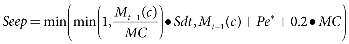 |
where:
Seep is the seepage depth for crop c on the current time-step (m)
Pe* is the effective rainfall depth for crop c in the current time-step (m)
dt is the model time-step (s)
Mt-1(c) is crop c soil moisture at the end of the previous time-step (m)
MC is the soil moisture capacity (m)
S is the seepage rate (m/s)
The process for updating the soil moisture for ponded and non-ponded crops differs. A crop is considered ponded when the pond minimum and maximum target levels are greater than zero. The process for ponded crops is based on maintaining a minimum pond target:
- Calculate trial updated soil moisture - Equation 33
- Calculate target - Equation 34
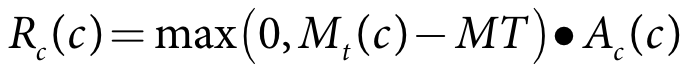
- Calculate runoff - Equation 35
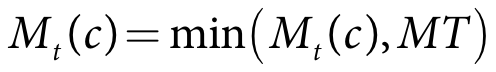
- Calculate final updated soil moisture - Equation 35.
| Equation 33 | 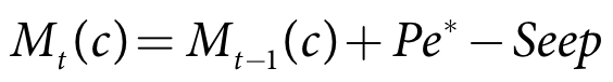 |
Equation 34 |
|

| Equation 35 |
|
| Equation 36 |
|
where:
Mt(c) is crop c soil moisture for the current time-step (m)
Mt-1(c) is crop c soil moisture at the end of the previous time-step (m)
Pe* is the soil rainfall depth for crop c in the current time-step (m)
Seep is the seepage depth for crop c in the current time-step (m)
Pondmax(c,t) is the user-specified current time-step maximum pond depth (m)
Pondmin(c,t) is the user-specified current time-step minimum pond depth (m)
MT is the current time-step target maximum pond depth for crop c (m)
MC is the soil moisture capacity (m)
CT(c) is theuser-specified crop tolerance for crop c (m)
Rc(c) is the runoff volume for crop c in the current time-step (m3)
Ac(c) is the area of crop c (m2)
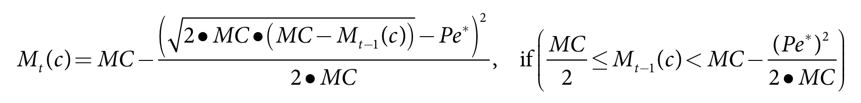
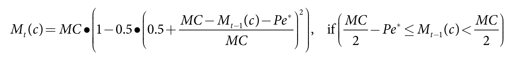
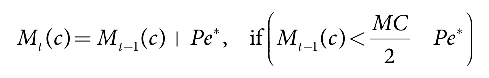
The process for non ponded crops allows for different soil moisture infiltration depending on the level of soil saturation. For fully saturated soil all rainfall will become runoff, for wet soil most of the rainfall runs off, for average soil moisture only a small amount runs of and for dry soil no rainfall runs off. The method is:
- Calculate trial crop soil moisture:
- When saturated - Equation 37
- When wet - Equation 38
- Under average conditions - Equation 39
- When dry - Equation 40
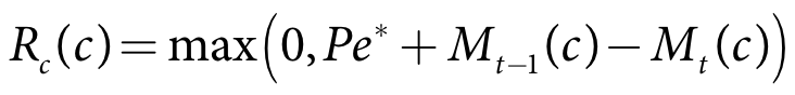
- Calculate trial runoff estimate - Equation 41
- Calculate final updated crop soil moisture - Equation 42
- Calculate final updated runoff - Equation 43.
Equation 37 | 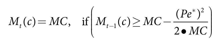 |
| Equation 38 |
|
| Equation 39 |
|
| Equation 40 |
|
| Equation 41 |
|
| Equation 42 |  |
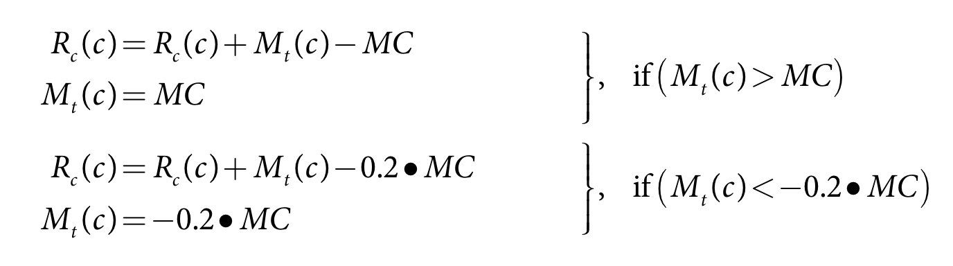 |
| Equation 43 |
|
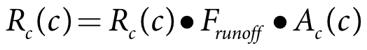
where:
Mt(c) is crop c soil moisture for the current time-step (m)
Mt-1(c) is crop c soil moisture at the end of the previous time-step (m)
MC is the soil moisture capacity (m)
Pe* is the effective rainfall depth for crop c in the current time-step (m)
Seep is the seepage depth for crop c in the current time-step (m)
Rc(c) is the runoff depth for crop c in the current time-step (m)
FRunoff is the runoff scaling factor
Ac(c) is the area of crop c (m2)
The soil moisture for fallow is maintained in two stores: the upper and lower fallow stores. The upper fallow store is firstly updated for rainfall, evapotranspiration and infiltration. Where the rainfall exceeds soil moisture levels all or a portion of the rainfall will appear as runoff. The lower fallow store is then adjusted for infiltration and seepage.
The effective rainfall on the fallow upper store (Equation 43) is the rainfall less fallow interception loss and fallow evaporation and is limited to the remaining soil moisture plus 20% of the moisture capacity of the soil (Lyall & Macoun Consulting Engineers, 1986)
| Equation 44 |  |
where:
Pe* is the soil rainfall depth for fallow on the current time-step (m)
P is the current rainfall rate (m/s)
dt is the model time-step (s)
Floss is the fallow interception loss (m)
KF is the current fallow evaporation factor
E0(t) is the current potential evapotranspiration rate (m/s)
FUMt-1 is upper fallow soil moisture at the end of the previous time-step (m)
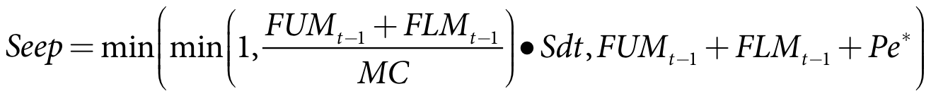
The infiltration to the lower fallow store is based on the upper fallow soil moisture content at the end of the previous time-step and is limited to previous moisture plus the effective rainfall and the airspace in the lower fallow store (see Equation 45) The seepage from the upper and lower fallow stores is based on the total fallow soil moisture content at the end of the previous time-step and is limited to the available soil moisture plus the effective rainfall (see Equation 46).
| Equation 45 | 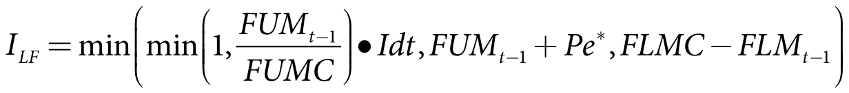 |
| Equation 46 |
|
where:
Seep is the seepage depth for fallow in the current time-step (m)
ILF is the infiltration to the lower fallow store (m)
I is the infiltration rate from the upper fallow to the lower fallow store (m/s)
S is the seepage rate from soil moisture stores (m/s)
Pe* is the effective rainfall depth for fallow in the current time-step (m)
dt is the model time-step (s)
FUMt-1 is upper fallow moisture at the end of the previous time-step (m)
FLMt-1 is lower fallow moisture at the end of the previous time-step (m)
FUMC is upper fallow soil moisture capacity (m)
FLMC is lower fallow soil moisture capacity (m)
MC is the combined upper and lower fallow soil moisture capacity (m)
Equation 47 and Equation 48. describe. The updating of the lower fallow moisture store.
| Equation 47 |  |
Equation 48 |
|
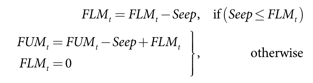
where:
Seep is the seepage depth for crop c on the current time-step (m)
ILF is the infiltration to the lower fallow store (m)
FUMt-1 is upper fallow soil moisture at the end of the previous time-step (m)
FLMt-1 is lower fallow soil moisture at the end of the previous time-step (m)
FUMt is upper fallow soil moisture at the end of the current time-step (m)
FLMt is lower fallow soil moisture at the end of the current time-step (m)
The upper fallow moisture store is updated in a similar manner to crops as detailed in Equation 37 through Equation 43 Note the upper fallow has a different runoff factor (Ffallow).
Updating the crop soil moisture for irrigation
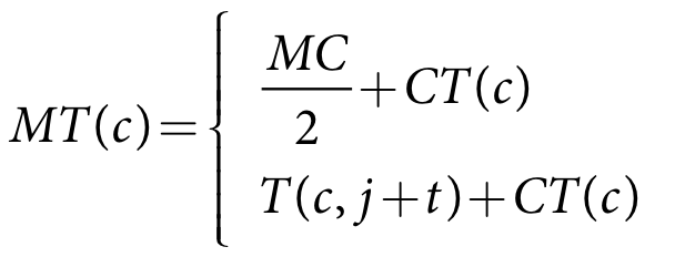
The crop is irrigated up to the soil moisture target plus an optional tolerance. This is detailed in Equation 49 (ponded), Equation 50 (non-ponded), Equation 51 (available water) and Equation 52 (moisture).
| Equation 49 |  |
Equation 50 |
|
| Equation 51 |
|

| Equation 52 |
|

where
MT(c) is the soil moisture target for crop c (m)
MC is the soil moisture capacity (m)
Pondmax(c,t) is current maximum pond depth (m)
CT(c) is the crop tolerance for crop c (m)
T(c,j+1) is the soil moisture target (when specified) on day (m)
EX(c) is the current extracted water for crop c (Equation 29) (m3)
Lret(c) is the return loss factor for crop c
Fret is the return loss factor
Lloss(c) is the on-farm loss factor for crop c
Floss is the on-farm loss factor
Lesc(c) is the escape loss factor for crop c
Fesc is the escape loss factor
AWc(c) is the current water available for crop c (m3)
M(c,t) is crop c soil moisture for the current time-step (m)
Losses and returns
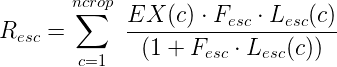
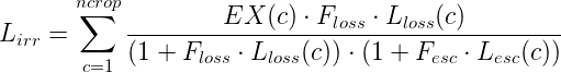
The on-farm escape, on-farm loss and irrigation return volumes are removed from the extracted volume prior to water being supplied to the crop. These are calculated using Equation 53 (escape return), Equation 54 (irrigation loss) and Equation 55 (Irrigation return), respectively.
| Equation 53 |
|
| Equation 54 |
|
| Equation 55 |
|

where:
Resc is the on-farm escape return volume (m3)
Lirr is the irrigation loss volume (m3)
Rirr is the irrigation return volume (m3)
EX(c) is the current extracted water for crop c (Equation 29) (m3)
Lret(c) is the return loss factor for crop c
Fret is the return loss factor
Lloss(c) is the on-farm loss factor for crop c
Floss is the on-farm loss factor
Lesc(c) is the escape loss factor for crop c
Fesc is the escape loss factor
The volume being returned to the water user is adjusted by the irrigation recycling efficiency Eret and is calculated as shown in Equation 56. Note the remainder is assumed to be lost.
| Equation 56 | 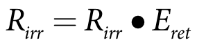 |
where:
Rirr is the irrigation return volume (m3)
Eret is the irrigation return efficiency
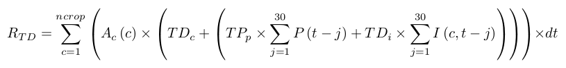
Two other kinds of return flows are available in the IQQM crop model: rainfall runoff returns and tile drainage. The runoff returns from crops have been described previously in Equation 35 and Equation 43 and fallow in equation Equation 44 The tile drainage function allows drainage to be defined in terms of a regression relationship with rainfall and irrigation over the previous 30 days. The amount of tile drainage return volume from crop areas is estimated as described in Equation 57 through Equation 59:
Equation 57 | 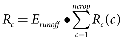 |
| Equation 58 |
|
| Equation 59 |
|

where:
Rc is the runoff return volume (m3)
Rc(c) is the runoff return volume (Equation 43) from crop c (m3)
Erunoff is the runoff recycling efficiency
RTD is the tile drainage return volume (m3)
Ac(c) is the area of crop c (m2)
ncrop is the number of crops
TDc is the tile drainage constant rate (m/s)
TDp is the tile drainage rainfall rate (m/s)
TDi is the tile drainage irrigation rate (m/s)
P(t-j) is the rainfall at time t-j (Equation 27)
I(c,t-j) is the water available for crop c at time t-j (Equation 28)
Rirr is the irrigation return volume (m3)
Rtot is the total return volume to the water user (m3)
On-farm storage reserve
The reserve to be held in the water user storage can be passed from the IQQM crop model to the water user. This allows the user to specify a reserve to be held as function of the area that is planted. This is calculated as shown in Equation 60.
| Equation 60 |  |
where:
OFSreserve is the volume to be held in reserve in the water user storage (m3)
Ac(c) is the area of crop c (m2)
ncrop is the number of crops
RES(c) is the reserve to be held for crop c (m)
Assumptions and constraints
The IQQM crop model assumptions and constraints are:
- Only available volume and antecedent conditions influence the area to plant. Other economic drivers are ignored;
- Crops never die. During the growing period of the crop if soil moisture levels reach zero for an extended period and water becomes available the soil moisture level will be topped up to the target soil moisture and evapotranspiration will occur;
- Evapotranspiration will cease when the soil moisture is drawn down by 20% of its capacity;
- The crop model has been designed to represent a group of farms and assumes the irrigation behaviour of a group of farms;
- The model assumes that all of the soil moisture is available to the crop irrespective of the stage of growth;
- Perennial crops or permanent plantings must be grown in the primary season. The area of this crop is influenced by the primary crop planting decision;
- The crop mix remains constant each year of the simulation; and
- Crops are planted on the same specified date each year of the simulation.
Input data
Refer to the Source User Guide for detailed data requirements and formats. The information that users need to provide is summarised in Table 1 through Table 9.
Table 1. Input parameters (planted area)
Parameter | Description | Units (default) | Range |
|---|---|---|---|
Atot | Maximum farm area | ha (100) | ≥0 |
DF | Proportion of area developed | % (100) | 0-100% |
Amax(p) | Maximum area of primary crop | ha (100) | 0≤Amax≤Atot•DF |
Amax(s) | Maximum area of secondary crop | ha (100) | 0≤Amax≤Atot•DF |
Table 2. Input parameters (planting decision)
Parameter | Description | Units (default) | Range |
|---|---|---|---|
Primary season decision date | day/month (1/10) | 1/1-31/12 | |
Secondary season decision date | day/month (1/3) | 1/1-31/12 | |
Risk function | yes/no (no) | ||
Risk function type | volume/area (area) | ||
TS | Antecedent inflows | ML/day (0) | ≥0 |
TSM | Antecedent monthly index (12 values) | ML (0) | ≥0 |
ALmax | Maximum expected volume or area | ML or ha (100) | |
Amin, Alimit | Minimum volume or area for planting (Vol or Area) | ML or ha (0) | ≥0 |
Amin | Threshold for planting (area based only) | Ha (0) | |
mw | Wet slope | ML/ML or ML/ha (1) | ≥ma |
bw | Wet intercept | ML or ha (0) | ≥ba |
iw | Wet index | (3) | ≥Ia |
ma | Average slope | ML/ML or ML/ha (1) | ≥md |
ba | Average intercept | ML or ha (0) | ≥bd |
ia | Average index | (2) | ≥Id |
md | Dry slope | ML/ML or ML/ha (1) | ≥0 |
bd | Dry intercept | ML or ha (0) | ≥0 |
id | Dry index | (1) | ≥0 |
Table 3. Input parameters (soil)
Parameter | Description | Units (default) | Range |
|---|---|---|---|
MC | Maximum available soil moisture | mm (200) | ≥0 |
FUMC | Upper soil moisture depth of fallow | mm (20) | ≥0 |
I | Infiltration rate from upper to lower fallow store | mm/d (0) | ≥0 |
S | Seepage from soil store | mm/d (0) | ≥0 |
Table 4. Input parameters (return flow)
Parameter | Description | Units (default) | Range |
|---|---|---|---|
Frunoff | Rainfall-runoff scaling factor | (1) | ≥0 |
Eret | Irrigation return water recycling efficiency | % (100) | 0≤Eret≤100 |
Erunoff | Rainfall runoff recycling efficiency | % (100) | 0≤Erunoff≤100 |
Table 5. Input parameters (climate)
Description | Units (default) | Range | |
|---|---|---|---|
E0(t) | Potential evaporation (time series) | mm/d (none) | ≥0 |
È0(j) | Average evaporation pattern (366 values) | mm/d (0) | ≥0 |
P | Rainfall (time series) | mm/d (none) | ≥0 |
Ploss | Crop interception loss | mm (0) | ≥0 |
Floss | Fallow interception loss | mm (0) | ≥0 |
Table 6. Input parameters (crop)
Parameter | Description | Units (default) | Range |
|---|---|---|---|
Crop factors | |||
Kcini | Initial crop factor | (0.3) | >0 |
Kcdev | Development crop factor | (0.3) | >0 |
Kcmid | Mid season crop factor | (1) | >0 |
Kclate | Late season crop factor | (1) | >0 |
Kcend | End season crop factor | (0.5) | >0 |
Initial stage | Day (30) | ≥0 | |
Development stage | Day (30) | ≥0 | |
Mid season stage | Day (60) | ≥0 | |
Late season stage | Day (30) | ≥0 | |
Kc(t) | Crop factor pattern (366 values) | (0) | ≥0 |
Lesc | Crop escape factor | (0) | ≥0 |
Lloss | Crop loss factor | (0) | ≥0 |
Lret | Crop irrigation return factor | (0) | ≥0 |
KF | Fallow crop factor | (0.4) | ≥0 |
Table 7. Input parameters (crop mix; values per crop)
Parameter | Description | Units (default) | Range |
|---|---|---|---|
Ec | Crop evapotranspiration efficiency | (1) | 0<Ec≤1 |
Start date | day/month (1/1) | 1/1-31/12 | |
Pc | Proportion of crop mix (Sum of all proportions = 1) | (0) | 0≤Pc≤1 |
CT | Crop tolerance | mm (0) | ≥0 |
s | Growing season | Primary/Secondary (Primary) | |
T | Crop soil moisture target pattern (daily pattern for crop) | mm (none) | 0≤T≤MC |
RES | OFS reserve volume pattern (Monthly or daily pattern) | ML/ha (none) | ≥0 |
Pondmin | Minimum pond level (daily pattern)* | mm (0) | ≥0 |
Pondmax | Maximum pond level (daily pattern)* | mm (0) | ≥0 |
* only for ponded crops
Table 8. Input parameters (efficiency)
Parameter | Description | Units (default) | Range |
|---|---|---|---|
Fesc | Farm escape factor | (1) | ≥0 |
Floss | Farm loss factor | (1) | ≥0 |
Fret | Farm Irrigation return factor | (1) | ≥0 |
Table 9. Input parameters (tile drainage, RTD)
Parameter | Description | Units (default) | Range |
|---|---|---|---|
Enable tile drainage | yes/no (no) | ||
TDi | Tile drainage irrigation factor | (0) | ≥0 |
TDc | Tile drainage coefficient | (0) | ≥0 |
TDp | Tile drainage rainfall factor | (0) | ≥0 |
Output data
A summary of IQQM crop model outputs is shown in Table 10.
Table 10. Summary of IQQM crop model outputs
Parameters | Default units |
|---|---|
Area shortfall | ha |
Average crop moisture | mm |
Crop demand | ML |
Crop opportunistic demand | ML |
Crop | |
Area | ha |
Moisture | mm |
Crop OFS reserve volume | ML |
Effective rain | mm |
Fallow | |
Area | ha |
Lower moisture | mm |
Total moisture | mm |
Upper moisture | |
Losses | |
Irrigation return loss | ML |
On-farm loss | ML |
Farm OFS reserve volume | ML |
Opportunistic crop demand | ML |
Resource available | ML |
Return flow | |
Crop runoff | ML |
Fallow runoff | ML |
Irrigation return | ML |
On-farm escape return | ML |
Tile drainage return | ML |
Total return flow | ML |
Sustainable area | ha |
Total crop area | ha |
Total seepage | mm/d |
Volume required | ML |
Water supplied by water user | ML |
Water supplied to crop | ML |
References
DIPNR (2004), IQQM Reference manual, Version 1.2, NSW Department of Infrastructure Planning and Natural Resources, NSW.
Lyall and Macoun Consulting Engineers (1986) WARAS Reference Manual, Version 1.0, prepared for the former Department of Water Resources, NSW
Allen, R.G., Pereira, L.S., Raes, D and Martin, M (1998) Crop evapotranspiration - Guidelines for computing crop water requirements FAO Irrigation and drainage paper 56 Food and Agriculture Organization of the United Nations, Rome ISBN 92-5-104219-5 Available at http://www.fao.org/docrep/X0490E/X0490E00.htm
Source User Guide