Note: This is documentation for version 4.11 of Source. For a different version of Source, select the relevant space by using the Spaces menu in the toolbar above
SMARG - SRG
Description and rationale
SMARG is a lumped conceptual rainfall runoff water balance model. The model provides daily estimates of surface runoff, groundwater discharge, evapotranspiration and leakage from the soil profile for the catchment as a whole. SMARG contains five water balance parameters and four routing parameters.
The documentation of this model is from Podger (2004) with some modifications to suit the needs of the SRG.
Scale
SMARG is a catchment scale model and operates at a daily time step.
Principal developer
The version of SMARG implemented in Source comes from the CRC for Catchment Hydrology Rainfall-Runoff Library (RRL), where it is referred to as the soil moisture and accounting model (SMAR) (O’Connell et al., 1970; Kachroo, 1992)
Scientific Provenance
SMARG is SMAR with modification to route surface runoff and the groundwater contribution to the stream separately (Kachroo and Liang, 1992). This modified model is also often referred to in the literature as SMAR rather than SMARG (e.g. Podger, 2004; Tuteja and Cunnane, 1999; Vaze et al., 2004).
Version
Source v2.10
Rainfall Runoff Library v1.0.5, June 25, 2004
http://www.toolkit.net.au/Tools/RRL
Dependencies
None.
Availability
Automatically provided with Source. SMARG is also available through the Rainfall Runoff Library (RRL) through http://www.toolkit.net.au/Tools/RRL.
Theory
SMARG consists of two components in sequence, a water balance component and a routing component. A schematic diagram of the SMARG model is shown in Figure 1. The model utilises input time series of daily rainfall and pan evaporation data to simulate stream flow at the catchment outlet. The model is calibrated against observed daily stream flow.
Figure 1. Structure of the SMARG rainfall-runoff model
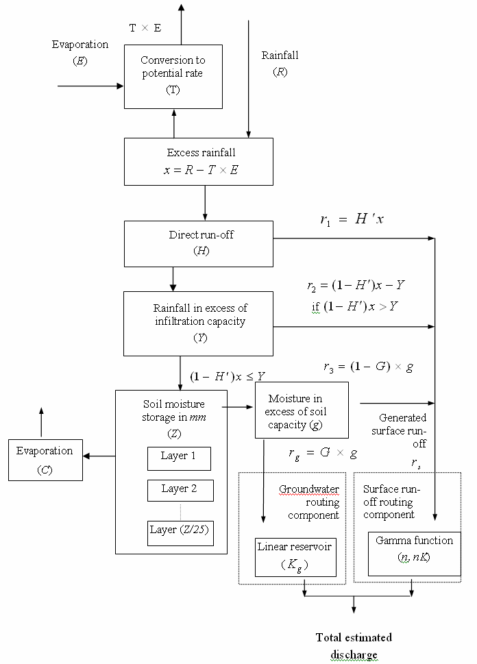
The water balance component divides the soil column into horizontal layers, which contain a prescribed amount of water (usually 25 mm) at their field capacities. Evaporation from soil layers is treated in a way that reduces the soil moisture storage in an exponential manner from a given potential evapotranspiration demand. The routing component transforms the surface runoff generated from the water balance component to the catchment outlet by a gamma function model form (Nash, 1960), a parametric solution of the differential routing equation in a single input single output system. The generated groundwater runoff is routed through a single linear reservoir and provides the groundwater contribution to the stream at the catchment outlet.
The surface run-off generated from the landscape is routed (attenuation and lag) to the catchment outlet using the linear cascade model of Nash (1960). The model was obtained as a general solution relating a given input of unit volume to a given output as in equation 1.
| Equation 1 | 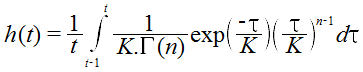 |
|---|
where:
t = simulation time-step (d);
τ = time (s);
K1 = K2 = ... ... = Kn = K are the storage coefficients of n linear reservoirs in cascade;
h(t) = ordinates of the pulse response function (d-1); and
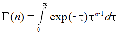 is the incomplete Gamma function (dimensionless).
It was shown by Nash (1960), that under constraints of conservation, stability, high damping and the absence of feedback, this two-parameter equation with n an integer and K positive, is almost as general a model as the differential equation of unlimited order. With additional flexibility obtained by allowing n to take fractional values, the impulse response of this equation has the ability to represent, adequately, almost all shapes commonly encountered in the hydrological context.
Water balance
The water balance component uses five parameters to describe the movement of water into and out of a generalised soil column under conditions of atmospheric forcing: C, Z, H, Y and T.
- The dimensionless parameter C regulates evaporation from the soil layers. Evaporation is assumed to vary as an exponential function of the form Ci-1, where C lies between 0 and 1 and i = 1,2,3… refers to the successive soil layers. That is, for a given potential evaporation the first layer can meet that demand at the potential rate, the second layer at a rate C1, the third layer at C2 etc, resulting in a reduction in the soil moisture store in an approximately exponential manner. The potential evapotranspiration rate from the top layer conceptually represents evapotranspiration from the interception storage and from the topsoil during periods of negligible capillary resistance.
- The parameter Z (mm) represents the effective moisture storage capacity of the soil contributing to the runoff generation mechanisms. Usually, each layer holds 25 mm at field capacity.
- The dimensionless parameter H is used to estimate the variable H’, the proportion of rainfall excess contributing to the generated runoff as saturation excess runoff or the Dunne runoff. H’ is obtained as a product of H and degree of soil saturation. Degree of soil saturation is defined as the ratio of available soil moisture in mm at time t (days) and 125 mm, which is the maximum soil moisture content of the first five layers.
- The parameter Y (mm·d-1) represents the infiltration capacity of the soil and is used for estimating the infiltration excess runoff (Hortonian runoff).
- The dimensionless parameter T is used to calculate the potential evapotranspiration from pan evaporation (E).
Generated surface runoff is calculated from the excess rainfall (rainfall minus potential evapotranspiration) as saturation excess runoff (shallow sub-surface flow) plus the Hortonian runoff and plus a proportion (1-G) of moisture in excess of the effective soil moisture storage capacity (g) (i.e. through flow). The remaining proportion (G) of the latter is the deep drainage component discharged from the groundwater system to the stream.
Routing
Groundwater and surface runoff, generated from the water balance component, are routed to simulate the associated lags between rainfall events and flow out of the catchment. The routing component has four parameters (n, nK, G, Kg), where the first two are for surface runoff and the remaining two are for groundwater discharge. The governing equations used in the routing component of SMARG are presented as follows (Kachroo and Liang, 1992).
Surface Runoff Routing
The total generated surface runoff is routed using a gamma function model form (i.e. based on equation 1) to obtain the daily total estimated discharge at the catchment outlet.
The generated surface runoff (rs mm·d-1) and the routed runoff (QrT mm·d-1) can be time averaged, as in equations (2) and (3), to represent the daily values.
| Equation 2 | 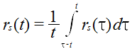 |
|---|
| Equation 3 | 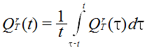 |
|---|
The linear model described by equation 4 (below) is the simplest representation of a causal, time invariant, relationship between an input function of time (generated runoff) and the corresponding output function (routed runoff). It is used in conceptual modelling, as a component, representing the routing or diffusion, effects of the catchment on those components of the rainfall hyetograph contributing to the outflow.
| Equation 4 | 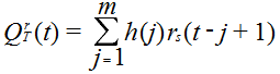 |
|---|
where:
m = memory of the pulse response function (d).
The parameter pair n and nK are chosen for optimisation, rather than n and K separately, because n is a ‘shape’ parameter and nK is the scale parameter. Expressed in this way, the two parameters are likely to be more independent than n and K would be separately, both of which contribute to the scale and to the shape, although in different ways.
Groundwater Discharge Routing
The mass balance equation for the groundwater system can be written as in equation 5:
| Equation 5 | 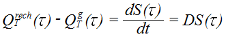 |
|---|
where:
QTrech = recharge to the groundwater system (mm.s-1).
QTg = discharge from the groundwater system (mm.s-1).
τ = time(s).
S(τ) = storage in the groundwater system (mm).
D = d/dt is the differential operator (s-1).
There are three basic components of discharge from the groundwater system:
- Discharge to the stream until a maximum threshold, after which discharge to land occurs following shallow watertable development.
- Discharge to the land surface that is locked in the landscape and is eventually lost to the atmosphere.
- Inter-basin transport, from the local groundwater system to the regional groundwater system.
In SMARG, the deep drainage component discharged from the groundwater system to the stream is routed through a linear reservoir with a large storage coefficient Kg. Two assumptions are made in treating the groundwater routing components as a single linear reservoir:
- Discharge to the land that does not eventually reach the river is negligible.
- Inter-basin transport from the local flow system to a regional groundwater system is substantially less than the discharge to the stream
Therefore, QTg is assumed to comprise groundwater discharge to the stream and to the land surface that eventually reaches the stream. The lag times between natural replenishment and groundwater discharge are substantial, and the groundwater system behaves like a highly damped system. This mechanism can be visualised as one of displacement whereby water from episodic drainage events is continually added at the bottom of the root zone and is removed from the groundwater system at a very slow rate, and can be represented as a linear reservoir with a large storage coefficient.
The pulse-response function for the groundwater component can be obtained in a manner analogous to equation 1, as in equation 6 (i.e. equation 1 with n and Γ(n) equal to 1; Vaze et al., 2004).
| Equation 6 | 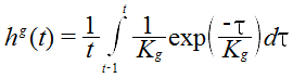 |
|---|
The recharge QTrech and the discharge QTg can be time averaged to mm·d-1 in an analogous manner to the generated surface runoff (rs) and the routed runoff (QrT), as in equations 2 and 3.
Data
Parameters
Parameters in SMARG and their default values are defined in Table 1.
Table 1. Parameters in SMARG and their default values
| Parameter | Description | Units | Default | Range |
|---|---|---|---|---|
| C | Evaporation coefficient | none | 0 | 0-1 |
| G | used to estimate the proportion of moisture in excess of soil moisture storage capacity recharging groundwater (and also discharged to the stream) | none | 0 | 0-1 |
| H | used to estimate the proportion of rainfall excess contributing to the generated runoff as saturation excess runoff or the Dunne runoff | none | 0 | 0-1 |
| Kg | Time lag parameter for groundwater routing | none | 0.01 | 0.01-200 |
| n | Surface runoff hydrograph ‘shape’ parameter (i.e. number of linear reservoirs) | none | 1 | 1-10 |
| nK | Surface runoff hydrograph ‘scale’ parameter (i.e. time lag parameter in Nash cascade model) | none | 1 | 1-10 |
| T | Ratio of potential evapotranspiration to pan evaporation | none | 0 | 0-1 |
| Y | Infiltration capacity of the soil | mm.d-1 | 0 | 0-100 |
| Z | Effective moisture storage capacity of the soil contributing to the runoff generation mechanisms | mm | 200 | 0-125 |
Output data
The variables listed in Table 2 can be recorded.
Table 2. Recorded variables
| Variable | Parameter | Frequency | Notes |
|---|---|---|---|
| PET | Potential evapotranspiration | time-step | |
| x | Excess rainfall | time-step | see Figure 1 |
| INF | Infiltration | time-step | Estimated from (1-H’)x (see Figure 1) |
| r1 | Direct runoff | time-step | see Figure 1 |
| r2 | Rainfall in excess of infiltration capacity (Hortonian runoff) | time-step | see Figure 1 |
| r3 | Moisture in excess of soil moisture capacity discharged to stream | time-step | see Figure 1 |
| r9 | Moisture in excess of soil moisture capacity recharging (percolating to) groundwater | time-step | see Figure 1 |
| rs | Generated surface runoff | time-step | see Figure 1 |
| QOUTsurf | Routed surface runoff (from gamma function) | time-step | see Figure 1 |
| QOUTgw | Routed groundwater runoff | time-step | see Figure 1 |
| SMStot | Soil moisture store contents (total of all layers) | time-step | see Figure 1 |
Reference list
Kachroo, R.K. (1992). River flow forecasting. Part 5. Applications of a conceptual model, Journal of Hydrology, 133: 141–178.
Kachroo, R.K. and Liang, G.C. (1992). River flow forecasting. Part 2. Algebraic development of linear modelling techniques, Journal of Hydrology, 133: 17–40.
Nash, J.E. (1960). A unit hydrograph study with particular reference to British catchments, Proceedings of the Institution of Civil Engineers, 17: 249–282.
O’Connell, P.E., Nash, J.E. and Farrel, J.P. (1970). Riverflow forecasting through conceptual models, part 2, the Brosna Catchment at Ferbane. Journal of Hydrology, 10: 317–329.
Podger, G.P. (2004). Rainfall Runoff Library User Guide, CRC for Catchment Hydrology.
Tuteja, N.K., and Cunnane, C. (1999). A quasi physical snowmelt run-off modelling system for small catchments, Hydrological Processes. 13(12/13): 1961–1975.
Vaze, J., Barnett, P., Beale, G., Dawes, W., Evans, R., Tuteja, N.K., Murphy, B., Geeves, G., and Miller, M. (2004). Modelling the effects of land-use change on water and salt delivery from a catchment affected by dryland salinity in south-east Australia, Hydrological Processes, 18: 1613–1637.