Bivariate Statistics SRG

Introduction

Many of the bivariate statistics available in Source are intended for the purpose of calibrating hydrological models, particularly for evaluating the fit between observed and modelled streamflow. The discussion below assumes that they are being used in this context. However, most of the statistics are generic and can be applied to evaluate the relationships other time series, or ordered variable, types.   

The main types of bivariate statistics available in Source are:

• Nash-Sutcliffe Efficiency (NSE)
• NSE of Log Data (NSE Log)
• Relative Bias
• Bias Penalty
• Pearson's Correlation Coefficient
• NSE of Flow Duration (Flow Duration)
• NSE of Flow Duration of Log Data (Log Flow Duration)
• Sum of Daily Flows, Daily Exceedance (Flow Duration) Curve and Bias (SDEB)

Source also offers a range of composite statistics that combine the NSE with other metrics. These are discussed in the section on Composite Bivariate Statistics Involving the NSE, are listed below:

• NSE Daily & Bias Penalty
• NSE Log Daily & Bias Penalty
• NSE Monthly & Bias Penalty
• NSE Daily & Flow Duration
• NSE Daily & Log Flow Duration

Each of the bivariate statistics is described below. For further information, the reader is referred to Vaze et al. (2011, Section 6), who discuss the use and interpretation of most of the bivariate statistics available in Source.

Treatment of Missing Data

It is common for hydrological time series to contain missing values and to have differing start and end dates. Generally, Source calculates bivariate statistics using only data from those time steps for which there are complete data pairs. The Bivariate Statistics tool in the Results Manager allows the user to calculate some statistics using all data (as opposed to just overlapping data). However, the results should be interpreted with caution.

Nash-Sutcliffe Efficiency (NSE) 

Definition

The NSE is a normalised metric that measures the relative magnitude of the model error variance compared to the measured data variance (Nash and Sutcliffe, 1970). It is defined as:

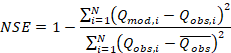
where: 

Q_obs,i    is the observed flow for time step i
Q_mod,i    is the modelled flow for time step i
N           is the number of time steps

The time step size is arbitrary.

Interpretation

The NSE can range between -∞ and 1, where:

• NSE = 1 corresponds to a perfect match between modelled and observed data
• NSE = 0 indicates that the model predictions are as accurate as the mean of the observed data
• NSE < 0 indicates that the mean of the observed data is a better predictor than the model

The NSE is sensitive to the timing of flow events and to extreme values. It is often applied on a daily time step (or shorter) to evaluate the model's ability to represent the timing of flow peaks and recession rates. Applying it on a longer time step, such as monthly, can be used to evaluate the fit to the pattern of flows without considering individual runoff events. The NSE is not suitable for evaluating a model's fit to low flows as the statistic will tend to be dominated by errors in the high flows.

The NSE is not very sensitive to systematic model over- or under-prediction, especially during low flow periods.

Discussion

An alternative, but equivalent, formulation of the NSE is:

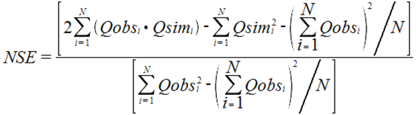
 This formulation obviates the necessity to calculate the average of the observed flows before evaluating the denominator in the traditional version.

NSE of Log Data (NSE Log)

Definition

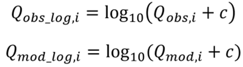
NSE Log is the standard NSE metric (Equation 1) applied to the logarithm of flow data:

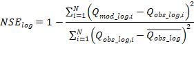
where:

c is a positive constant equal to the maximum of 1 ML and the 10^th percentile of the observed flow
other terms are as defined in Equation 1

As with the standard NSE, the time step size is arbitrary. The NSE Log cannot be applied to time series with negative values, as the logarithm of a number less than or equal to zero is undefined.

Interpretation

Using the logarithm of flows has the effect of reducing the sensitivity of the metric to high flows and increasing the sensitivity to low and mid-range flows. For this reason, NSE Log is often used for model calibration when low-flow performance is important. The use of the constant c de-emphasises very small flows, which tend to be unreliable, and avoids numerical problems with attempting to calculate the logarithm of zero flows.

The NSE Log can range between -∞ and 1 and the interpretation is the same as for the NSE, but applied to log data.

Relative Bias

Definition

The relative bias measures the magnitude of the model errors relative to the magnitude of the observations. It has the form:

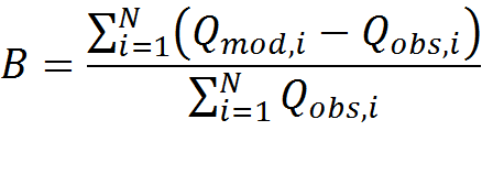
where:

Q_obs,i    is the observed flow for time step i
Q_mod,i    is the modelled flow for time step i
N           is the number of time steps

Interpretation

The relative bias, B, ranges from -∞ to +∞, where:

• B < 0 indicates that the modelled data underestimates the observed data
• B = 0 indicates that the model is unbiased
• B > 0 indicates that the modelled data underestimates the observed data

The relative bias measures the overall error in the volume of modelled flow, it does not measure the model's fit to the timing of flows (Vaze et al., 2011).

Discussion

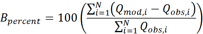
Common variations of the relative bias are to express it as a percent and/or as an absolute value. The bias in the modelled values expressed as a percent of the observed flow volume is defined as:

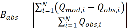
 The absolute value of the relative bias is defined as:

Bias Penalty

Definition

The bias penalty is a log transformation of the absolute value of the relative bias. It was proposed by Viney et al. (2009) and is defined as:

where B is the relative bias, as defined in Equation 4.

Interpretation

The bias penalty ranges from 0 to +∞, where a value of 0 indicates that the model is unbiased.
 
In Source, the bias penalty is always used in combination with the NSE and is not available on its own. It is designed to be used in model calibration to penalise biased solutions. Refer to Viney et al. (2009) for a discussion of the advantages of the bias penalty compared to the absolute value of the relative bias.

Pearson's Correlation Coefficient

Definition

Pearson's correlation coefficient measures the linear correlation between two variables. The sample Pearson's correlation coefficient is given by:

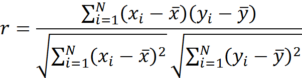
where:

x_i is the value of time series x at time step i
y_i is the value of time series y at time step i

The time step size is arbitrary. Pearson's correlation coefficient is symmetric, meaning that the value will be the same regardless of which time series is defined as x and which as y.

Interpretation

Pearson's correlation ranges from -1 to 1 where:

• r = -1 indicates perfect negative correlation
• r = 0 indicates that there is no correlation between the two variables
• r = +1 indicates perfect positive correlation

Pearson's correlation is sensitive to the relative magnitude of data points in a time series, but not the absolute magnitude. Two time series can have a perfect correlation if they have the same "shape", even if the values are different.

NSE of Flow Duration (Flow Duration)

Definition

The Flow Duration is calculated by sorting the observed and modelled data values in increasing order and then calculating the NSE (Equation 1) of the sorted data.

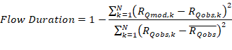
where:

R_Qobs,k is the k'th ranked observed flow of a total of N ranked flows R_Qsim,k is the k'th ranked modelled flow of a total of N ranked flows

It can be applied for any time step size.

Interpretation

The Flow Duration measures the fit to the distribution of flow magnitudes and does not consider the timing of flows. It is sensitive to high flows and less sensitive to low flows.

NSE of Flow Duration of Log Data (Log Flow Duration)

Definition

The Log Flow Duration is calculated applying the Flow Duration to log transformed data:

Interpretation

The Log Flow Duration measures the fit to the distribution of flow magnitudes and it is sensitive to low and mid-range flows.

Sum of Daily Flows, Daily Exceedance (Flow Duration) Curve and Bias (SDEB)

Definition

The SDEB metric was proposed by Lerat et al. (2013), based on a function introduced by Coron et al. (2012). It combines three terms:

1. the sum of errors on power transformed flow, 
2. the same sum on sorted flow values and 
3. the relative simulation bias.

The SDEB equation is:

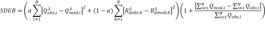
where:

α is a weighting factor set to 0.1

λ is an exponent set to 0.5

N is the number of time steps

Q_obs,i is the observed flow for time step i

Q_mod,i is the modelled flow for time step i

R_Qobs,k is the k'th ranked observed flow of a total of N ranked flows

R_Qsim,k is the k'th ranked modelled flow of a total of N ranked flows

The SDEB metric is designed to be applied to daily data.

Interpretation

The SDEB ranges from 0 to +∞, where a value of 0 indicates a perfect fit between modelled and observed data.

The coefficient α and the power transform λ are used to balance the three terms within the objective function.

• The weighting factor α is used to reduce the impact of the timing errors on the objective function. This type of error can have a significant effect on the first term in equation (X), where a slight misalignment of observed and simulated peak flow timing can result in large amplitude errors. The second term is based on sorted flow values, which remain unaffected by timing errors. By way of example, in their study of the Flinders and Gilbert Rivers in Northern Australia, Lerat et al. (2013) used values of α of 0.1 for the Flinders calibration and 1.0 for the Gilbert calibration.
• Using values of power transform λ of less than 1 has the effect of reducing the weight of the errors in high flows, where the flow data are known to be less accurate. Lerat et al. (2013) found that a power transform of ½ led to the best compromise between high and low flow performance in their project. This value has been adopted in Source.

Composite Bivariate Statistics Involving the NSE

Introduction

Often, when comparing two streamflow hydrographs or other time series data, no single metric measures all the characteristics of interest. Model calibration is usually performed using a composite objective function that combines two or more individual metrics. The SDEB equation is an example. Source also offers a number of composite statistics that involve various combinations of the NSE. These are:

• NSE Daily & Bias Penalty
• NSE Log Daily & Bias Penalty
• NSE Monthly & Bias Penalty
• NSE Daily & Flow Duration
• NSE Daily & Log Flow Duration

Some of the composite statistics allow the user to choose a weighting that determines the relative importance of each metric in the overall function.

NSE Daily & Bias Penalty

Definition

where:

NSE Daily is the NSE of daily flows as defined in Equation 1
Bias Penalty is defined in Equation 7

Interpretation

The NSE Daily & Bias Penalty function is designed to ensure that a model is calibrated primarily to optimise NSE while ensuring a low bias in the total streamflow. However, the function will be strongly influenced by moderate and high flows and by the timing of runoff events, and can result in poor fits to low flows.

NSE Log Daily & Bias Penalty

Definition

where:

NSE Log Daily is the NSE of the logarithm of daily flows, as defined in Equation 3
Bias Penalty is defined in Equation 7

Interpretation

The NSE Log Daily & Bias Penalty function is similar to the NSE Daily & Bias Penalty, but the use of the logarithm of flows puts an increased emphasis on low-flow performance.

NSE Monthly & Bias Penalty

Definition

where:

NSE Monthly is the NSE of monthly flows, as defined in Equation 1
Bias Penalty is defined in Equation 7

Note that, the aggregation of daily flows to monthly may be performed differently in different areas of Source. The Calibration Wizard, for example, uses the sum of the daily modelled and observed flows for each month.

Interpretation

The NSE Monthly & Bias Penalty function is similar to the NSE Daily & Bias Penalty, but the use of monthly flows means that it is not sensitive to the timing of individual runoff events.

NSE Daily & Flow Duration

Definition

where:

a is a user-defined weighting factor (0 ≤ a ≤ 1)
NSE Daily is the NSE of daily flows as defined in Equation 1
Flow Duration is defined in Equation 9

Interpretation

The NSE Daily & Flow Duration function is designed to balance a model's fit to the timing (and magnitude) of flow events and the overall distribution of flow volumes. It is sensitive to high flows and less sensitive to low flows. The user can choose the relative importance of the two objective function components.

NSE Daily & Log Flow Duration

Definition

where:

a is a user-defined weighting factor (0 ≤ a ≤ 1)
NSE Daily is the NSE of daily flows as defined in Equation 1
Log Flow Duration is defined Equation 9 and Equation 10

Interpretation

The NSE Daily & Log Flow Duration function is similar to the NSE Daily & Flow Duration. It puts greater emphasis on the distribution of low flow volumes.

References

Coron, L., V. Andrassian, P. Perrin, J. Lerat, J. Vaze, M. Bourqui and F. Hendrickx (2012) Crash testing hydrological models in contrasted climate conditions: an experiment on 216 Australian catchments. Water Resources Research, 48, W05552, doi:10.1029/ 2011WR011721.

Lerat, J., C.A. Egan, S. Kim, M. Gooda, A. Loy, Q. Shao and C. Petheram (2013) Calibration of river models for the Flinders and Gilbert catchments. A technical report to the Australian Government from the CSIRO Flinders and Gilbert Agricultural Resource Assessment, part of the North Queensland Irrigated Agriculture Strategy. CSIRO Water for a Healthy Country and Sustainable Agriculture flagships, Australia.

Nash, J.E. and J.V. Sutcliffe (1970) River flow forecasting through conceptual models part I — A discussion of principles. Journal of Hydrology, 10 (3), 282–290.

Vaze, J., P. Jordan, R. Beecham, A. Frost, G. Summerell (2011) Guidelines for rainfall-runoff modelling: Towards best practice model application. eWater Cooperative Research Centre, Canberra, ACT.  ISBN 978-1-921543-51-7. Available via www.ewater.org.au.

Viney, N.R., J-M. Perraud, J. Vaze, F.H.S Chiew, D.A. Post and A. Yang (2009) The usefulness of bias constraints in model calibration for regionalisation to ungauged catchments. In: 18th World IMACS Congress and MODSIM09 International Congress on Modelling and Simulation, July 2009, Cairns: Modelling and Simulation Society of Australian and New Zealand and International Association for Mathematics and Computers in Simulation: 3421-3427.