Note: This is documentation for version 4.11 of Source. For a different version of Source, select the relevant space by using the Spaces menu in the toolbar above
Chart Statistics
Single result
If a single time series is selected from the left-hand tree menu of the Results Manager window, the statistics tab will show univariate statistics (Figure 1). Univariate statistics provide information on a single result and are intended to summarise and reveal patterns in that result.
For statistics for a single result, you can:
- Choose the period type (Table 1) used to calculate the statistics from the drop-down menu;
- Change the Water Year Start from the default date (the default is set in Project Options);
- View the result used to calculate the statistics under Data;
- View the statistics themselves.
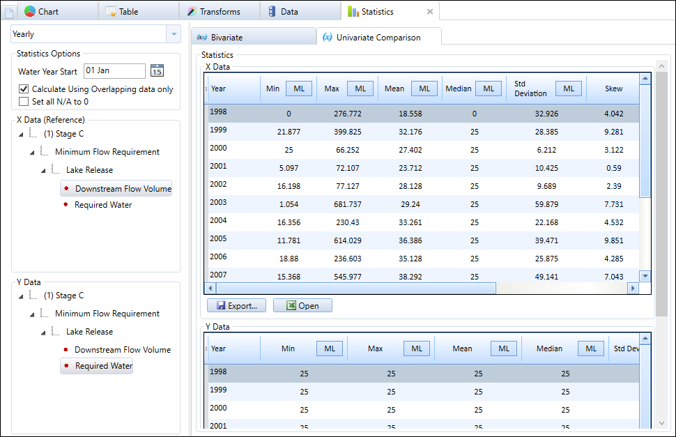
Multiple results
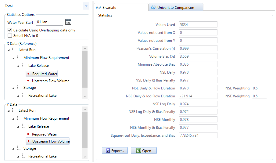
For multiple results in a custom chart, the statistics tab shows both univariate comparison (Figure 2) and bivariate statistics (Figure 3) for two of the results in the chart:
- Univariate comparison statistics are the same as univariate statistics for a single result, except that by default the statistics are only calculated from data that overlaps between the two results (see Table 2). To calculate univariate statistics for all data in each result, disable Calculate using overlapping data only.
- Bivariate statistics compare two results for the purpose of determining empirical relationships between them.
For statistics of multiple results, you can also:
- Toggle on or off two Statistics Options for how the two results are compared (Table 3);
- View and change the result used as the X Data (reference) and the Y Data for statistic calculations (in Figure 2, this is Downstream Flow Volume); and
- Select to view either Univariate Comparison or Bivariate statistics for the two results.
Table 1. Basic statistical analysis, period types
| Period type | Description |
|---|---|
| Total | Provides statistics for the entire run. This is the default period. |
| Yearly summary | Provides annual statistics, with one row for each year in the run. |
| Monthly summary | Provides monthly statistics by combining the data for each month, regardless of the year. There are 12 rows, one for each calendar month. For example, the January row displays statistics calculated from data for every January for all years in the run. |
| MonthxYear summary | Provides monthly statistics by month and year, with one row for each month-year pair in the run. For example, December 1999, January 2000, February 2000 ... etc. |
Table 2. Multiple results, parameters
| Parameter | Description | Default |
|---|---|---|
| Calculate using overlapping data only |
| Enabled |
| Set all N/A to 0 |
| Disabled |
Figure 1. Univariate statistics, single result.
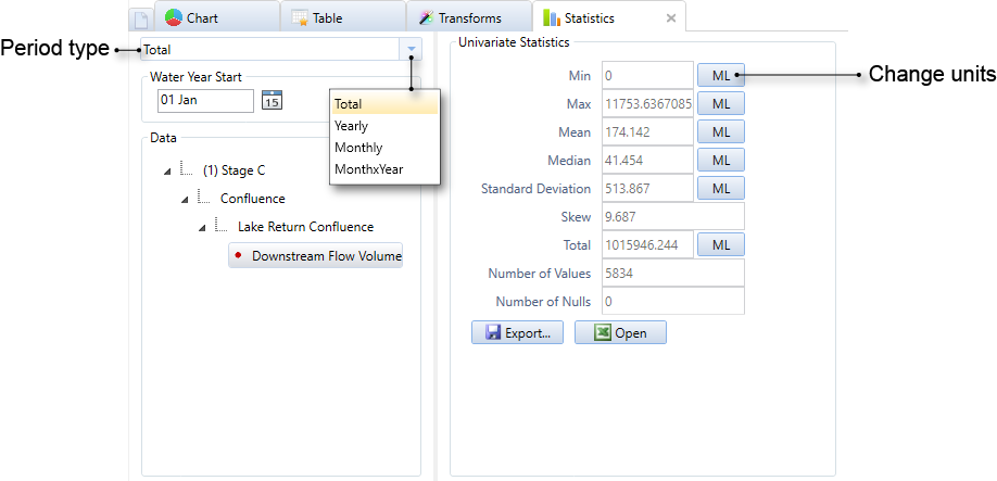
Figure 2. Univariate statistics, multiple results, yearly summary
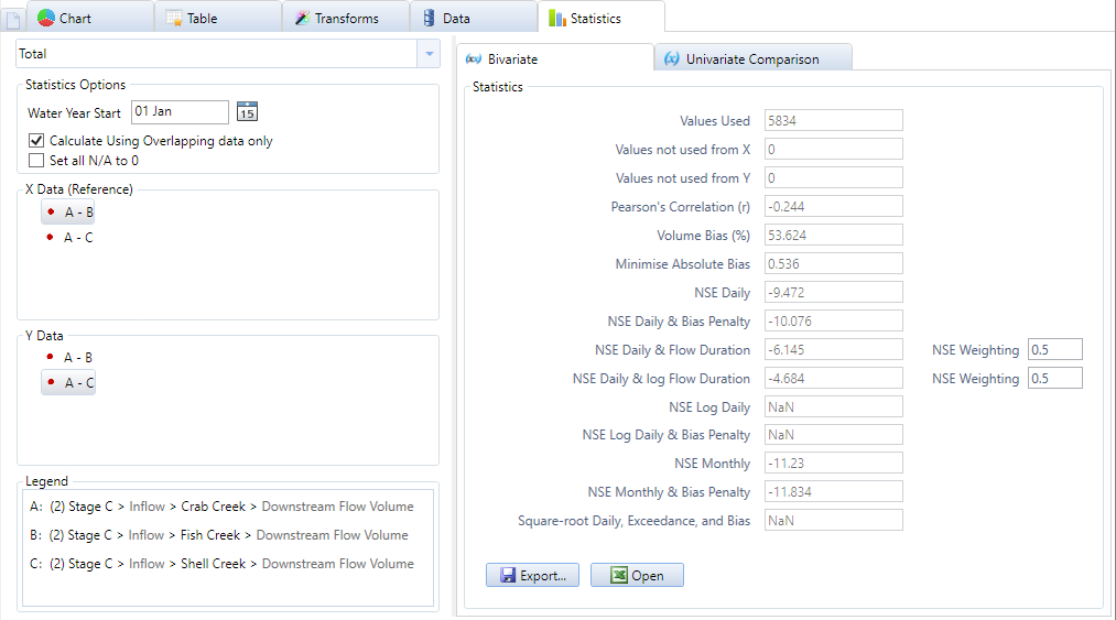
Naming conventions of difference, double mass and scatter statistics
If you have a custom chart with a chart type of difference, double mass or scatter, then the following naming conventions are used in the statistics tab (Figure 3):
- Each result in the custom chart is given a letter. This is shown in a Legend in the bottom left of the statistics tab.
- The series used as a reference in the chart is always given letter A. To change the reference series, go to the Chart view then select Chart Settings » Charts and modify Chart Type Reference Series.
- Under X Data (Reference) and Y (Data), the results are listed using the letters to represent each result.
For example, in Figure 3, A - B corresponds to the difference between Crab Creek's Downstream flow volume (result A) and Fish Creek's Downstream Flow Volume (result B).
Figure 3. Statistics, Difference Chart Type
Univariate statistics
You can view univariate statistics for a single result (as shown in Figure 1) or for each individual result when multiple results are combined (Figure 2). A brief description of each univariate statistic is given in Table 1, for more detailed information see Univariate Statistics SRG.
Table 1. Univariate Statistics
Statistic | Definition | Example for |
|---|---|---|
Minimum | Minimum value in the time series. | 0 |
Maximum | Maximum value in the time series. | 9 |
Number of Values | The number of values in the time series, not including nulls. | 6 |
Number of Nulls | The number of nulls, either missing values or values entered as -9999. These values are ignored in all other univariate statistics. | 1 |
Total | The sum of all values in the time series. | 27 |
Mean | The sum of all values in the time series divided by the number of values, | 5 |
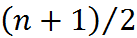
Median | The middle value in the sorted list of all values in a time series. For n values, the middle value is | 4 |
Standard Deviation | How widely values in the time series vary from the mean. See Standard Deviation. | 3.89 (to 2 decimal places) |
Skew | The skewness of the distribution of values in the time series. See Skew. | 0.23 (to 2 decimal places). |
Bivariate statistics
When two or more results are in a custom chart, a set of bivariate statistics is automatically generated and can be viewed on the Bivariate Statistics tab (Figure 4). A brief description of each bivariate statistic is given in Table 4, where:
- NSE (Nash-Sutcliffe Efficiency) measures the relative magnitude of the model error variance compared to the measured data variance. It can be applied at any time step size (eg. daily, monthly). See Bivariate Statistics SRG - Nash-Sutcliffe Efficiency
- The NSE of Flow Duration measures the NSE of the modelled and observed flow duration curves. It can be applied at any time step size (eg. daily, monthly). See Bivariate Statistics SRG - Flow Duration.
- Relative Bias measures the magnitude of the model errors relative to the magnitude of the observations. See Bivariate Statistics SRG - Relative Bias.
- Bias Penalty is log transformation of the absolute value of the relative bias. In Source, the bias penalty is always used in combination with the NSE and is not available on its own. It is designed to be used in model calibration to penalise biased solutions. See Bivariate Statistics SRG - Bias Penalty.
For more detailed information on bivariate statistics, see Bivariate Statistics SRG.
Parameter selection for bivariate statistics is the same as for a univariate comparison. If you select any period type other than Total, or you have disabled Calculate using overlapping data only and your start and/or end dates do not match, a subset of the statistics are available:
- Pearson's Correlation (r);
- NSE Daily;
- Volume Bias (%);
- Values used; and
- Values not used.
Table 4. Bivariate Statistics
Statistic | Definition | Scientific Reference Guide entry | Range |
|---|---|---|---|
Values Used | The number of time steps for which there are complete data pairs ie. both the X data and Y data time series have values. These pairs are used to calculate the bivariate statistics. Time steps where either series has missing values are not used. | 0 to +∞ | |
Values not used from X | The number of time steps in the X Data series that are not used in bivariate statistics calculations because either the X data or the Y data have missing values for those time steps. | 0 to +∞ | |
Values not used for Y | The number of time steps in the Y Data series that are not used in bivariate statistics calculations because either the X data or the Y data have missing values for those time steps. | 0 to +∞ | |
Pearson's Correlation (r) | Pearson's correlation coefficient measures the linear correlation between two variables. Pearson's correlation coefficient is symmetric, meaning that the value will be the same regardless of which time series is defined as X data (reference) and which as the Y data. | Pearson's Correlation Coefficient | -1 to 1 |
Volume Bias (%) | Relative bias expressed as a percentage. | Relative Bias | -100 to 100 |
Minimise Absolute Bias | The absolute value of the relative bias. | Relative Bias | 0 to +∞ |
| NSE Daily | The NSE for using a daily time step. | Nash-Sutcliffe Efficiency | -∞ to 1 |
NSE Daily & Bias Penalty | The difference between NSE daily and the Bias Penalty. | NSE Daily & Bias Penalty | -∞ to 1 |
NSE Daily & Flow Duration | Combines the NSE Daily and Flow Duration using a user-defined weighting factor. | NSE Daily & Flow Duration | -∞ to 1 |
| NSE Daily & log Flow Duration | Combines the NSE Daily and log Flow Duration using a user-defined weighting factor. Log flow duration is the NSE of flow duration of the logarithm of data, calculated using a daily time step. | NSE Daily & log Flow Duration | -∞ to 1 |
| NSE Log Daily | The NSE of the logarithm of data, using a daily time step. | NSE of Log Data | -∞ to 1 |
| NSE Log Daily & Bias Penalty | The difference between NSE Log daily and the Bias Penalty. | NSE Log Daily & Bias Penalty | -∞ to 1 |
| NSE Monthly | The NSE using a monthly time step | Nash-Sutcliffe Efficiency | -∞ to 1 |
| NSE Monthly & Bias Penalty | The difference between NSE monthly and the Bias Penalty. | NSE Monthly & Bias Penalty. | -∞ to 1 |
| Square-root Daily, Exceedance and Bias | Combines three terms, the sum of errors on power transformed flow, the same sum on sorted flow values, and the relative simulation bias. | SDEB | 0 to +∞ |
Figure 4. Bivariate statistics, Total period
MUSIC volumetric ratio statistic
In MUSIC Results Manager, is an additional bivariate statistic, Volumetric Ratio, which can be used to calculate the volumetric ratio between two flows, for example, pre and post development outflow. For each flow, the user chooses a threshold, and the area between the curve and the threshold is calculated. The ratio between these two areas is the Volumetric Ratio:
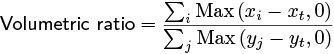
where xi is the ith value of the flow series x, xt is the user-defined threshold value for x, yj is the jth value of the flow series y, and yt is the user-defined threshold for y.
This statistic can be used to calculate several useful parameters such as Volumetric runoff coefficients and Stream Erosion Index (SEI). To calculate SEI, it is necessary to know the flow threshold (critical flow) below which no erosion is expected to occur within a waterway. This threshold can be represented (EarthTech, 2005) as a percentage of the pre‐development two-year ARI peak flow at the location in question. The percentage depends on the stream bed material and usually varies between 10 – 50%. The pre-development two-year ARI peak discharge can be estimated using flood frequency analysis or the rational method as described in Australian Rainfall and Runoff (Pilgrim, D.H., 2001). Flux Files containing the pre- and post-development outflows can be generated from MUSIC model run. SEI can be calculated by creating a custom chart in Results Manager where X data is the post-development outflow, Y data is the pre-development outflow, and both the X data and Y data threshold values are manually set to the value of critical flow using the appropriated fields next to the volumetric ratio.
Although Results Manager can calculate a volumetric ratio for any two data series, currently this statistic supports data expressed as either volume (eg. ML) or rate (eg. m3/s).