Note: This is documentation for version 4.11 of Source. For a different version of Source, select the relevant space by using the Spaces menu in the toolbar above
Groundwater Analytical Tool - GAT
Contents
Introduction
Source's Groundwater Analytical Tool (GAT) is a collection of modules and protocols/guidelines that simulate the exchange of groundwater and salt between rivers and the underlying groundwater systems. The module determines the exchange flux of water between a river and the underlying aquifer for each link of Source at each time-step. The estimated flux accounts for interactions between groundwater and surface water along the entire length of the link. The direction of flux can either be from the river to aquifer or vice versa, that is, the river either loses water to the groundwater system or it gains water from the groundwater system.
The various components of exchange flux may be calculated within Source or they can be imported as a time series from field monitoring. The exchange fluxes may include the following components:
- Continuous natural exchange between the river and the aquifer, which is driven by the head difference;
- Flux out due to evapotranspiration;
- Flux out due to groundwater pumping;
- Flux in due to irrigation and diffuse recharge; and/or
- Exchange fluxes during (within bank and overbank) flood events.
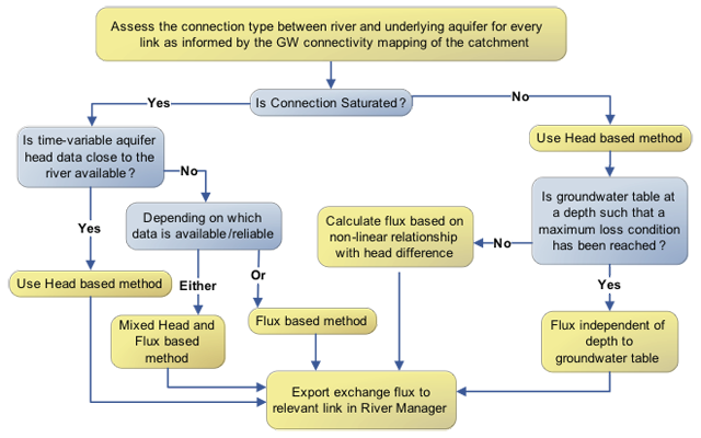
The process for selecting the appropriate methodology to estimate GW-SW exchange flux is mainly dictated by the type of connection between a river and the underlying aquifer, and is influenced by data availability. A decision-making flow chart (shown in Figure 1) is a guide in selecting the appropriate methodology for any situation.
Figure 1. GW-SW decision-making flowchart
Configuring groundwater in Source
Exchange fluxes are assigned to a Source link once storage routing has been enabled on the link (refer to Types of links routing). Use the link's feature editor (shown in Figure 2) to configure groundwater on a storage routing link.
Figure 2. Storage link routing, Groundwater
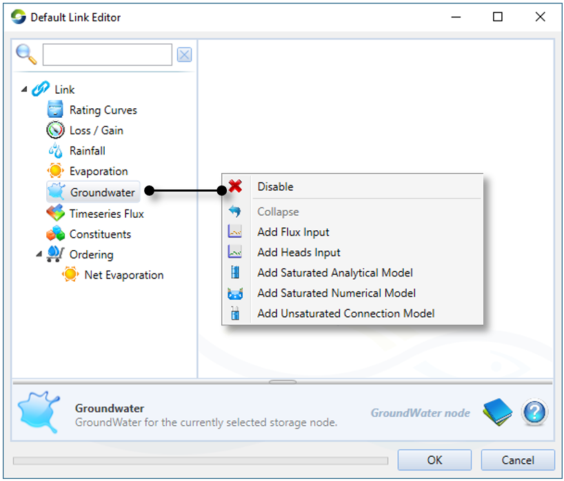
Types of groundwater models
There are four types of groundwater models which can be configured in Source; these are described next.
Flux input
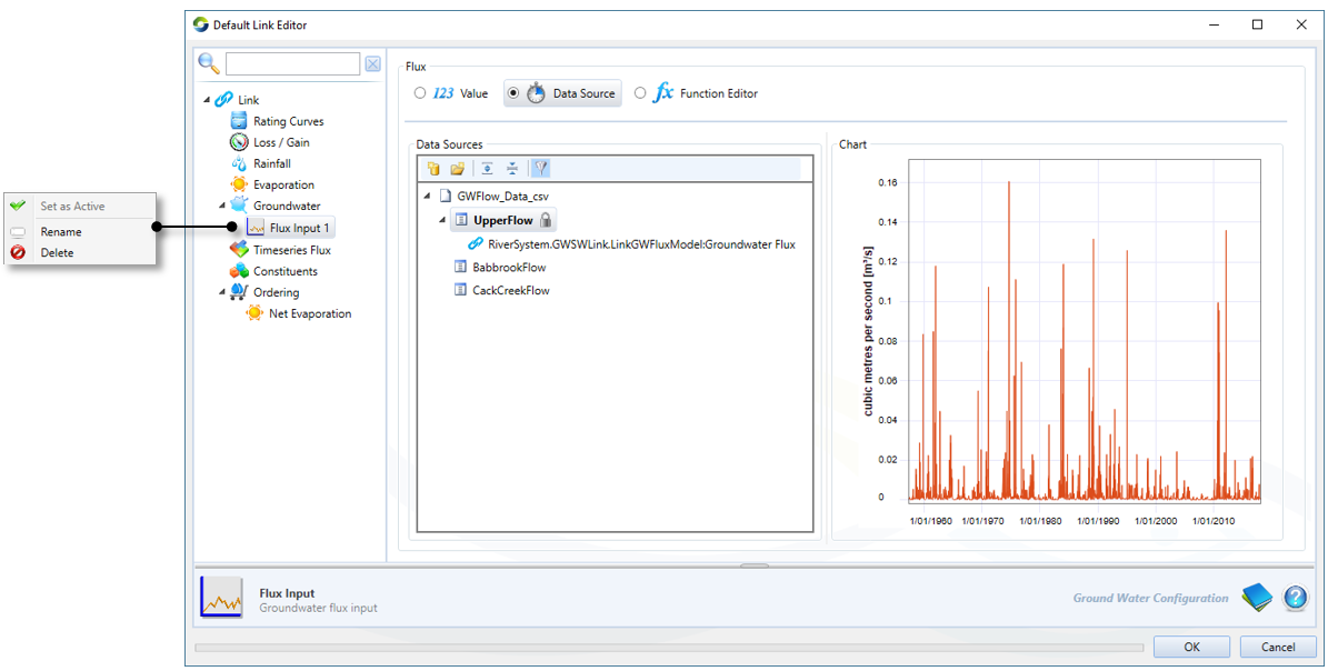
This represents the daily exchange flux between the reach and its aquifer, which can be specified as a single value, a time series (using Data Sources), or via a function using the Function Editor (Figure 3). Note that flux values can be both positive and negative, so the reach alternates between gaining and losing.
Figure 3. Groundwater, Flux Input
Heads input
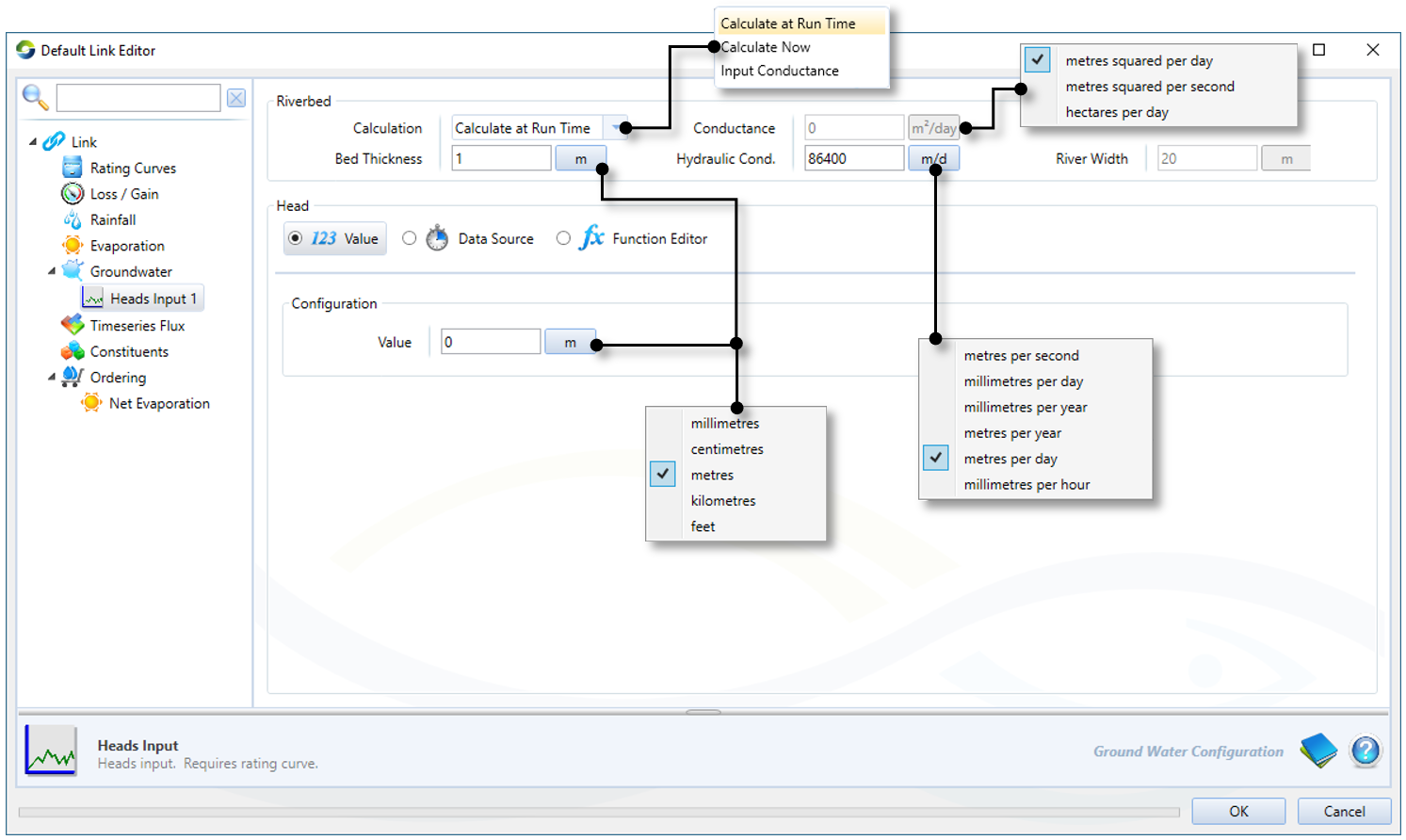
One method for estimating the groundwater flux is based on knowledge of the head difference between the river stage and the water table in the underlying aquifer. The Heads Time Series input model (Figure 4) uses the head difference between the current calculated river stage height (from rating curve and link level) and the interpolated groundwater head (from time series) to calculate groundwater flux.
A groundwater head value that is larger than the current stream height generates a flux from the aquifer to the stream (a negative flux) and a groundwater head value that is lower than the stream height generates a flux from the stream to the aquifer (a positive flux).
To configure Heads Input in Source, you need:
- A rating curve to determine river stage height from river discharge (refer to Link rating curve) and a stream (link) height;
- A conductance value (either set or calculated prior to run time, or calculated dynamically at run time); and
- A time series of groundwater heads covering the period of simulation (which can be specified as a single value, via a file using Data Sources, or via a function using the Function Editor).
Figure 4. Groundwater, Heads Time Series Input
Unsaturated connection
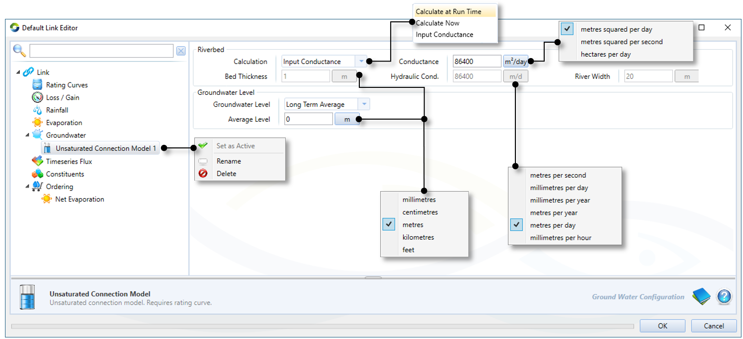
The Unsaturated Connection model (Figure 5) uses the head difference between the calculated river stage height (from the rating curve and link level) and groundwater head level specified.
There are three main steps to configuring the model:
- Load a rating curve and set stream (link) height. When using multiple rating curves, it is important that each curve has a unique start date to ensure that the model matches the current time-step with the relevant rating curve. The model gives a warning if a rating curve has the same start date;
- Enter a conductance value (similar to Heads Time Series Input); and
- Set the groundwater level as a long term average groundwater level, or via a simple forecast model. For an unsaturated connection model, the groundwater level must always be less than the river water level.
Under unsaturated conditions, the groundwater head value cannot be larger than the current stream height. Groundwater head is always below the stream bed level under unsaturated conditions.
Figure 5. Groundwater, unsaturated
Saturated Connection
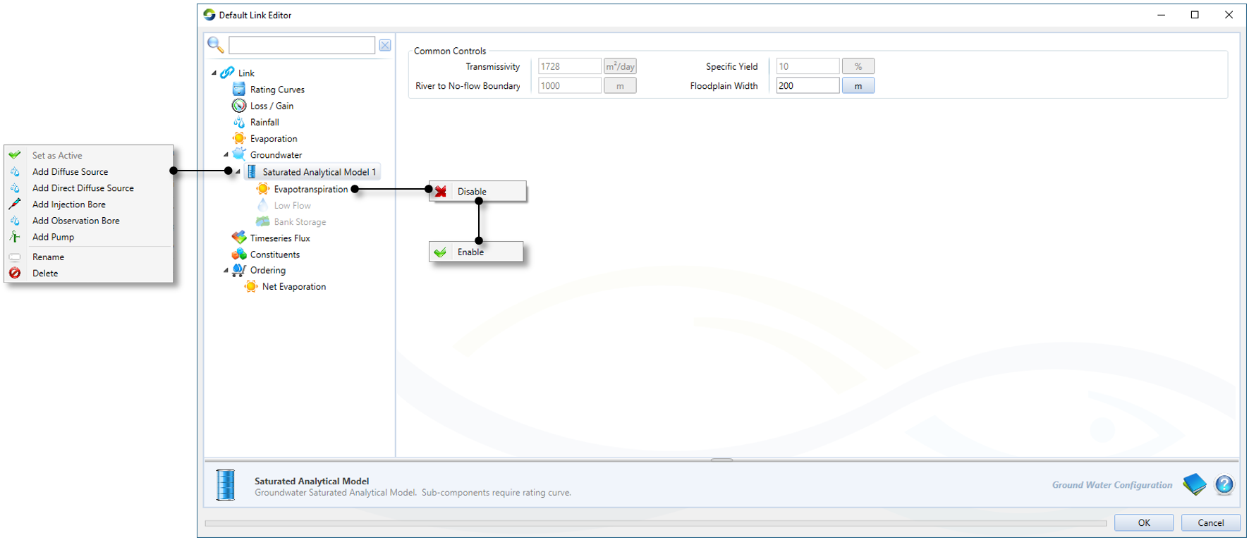
In a Saturated Connection model (shown in Figure 6), you may select any of the eight distinct groundwater and floodplain processes to run simultaneously. At each time-step the model evaluates the impacts of each selected process and uses assumed linearity and superposition to aggregate the impacts and calculate a flux. It is the most complex of all the groundwater models.
This model contains eight processes that can be enabled or disabled using the contextual menus shown in Figure 6. More detail is provided about them in the next section.
The parameters for the saturated connection model fall into one of two categories:
- Shared ones (labelled Common Controls in Figure 6 and defined in Table 1). These parameters are only set once per link and are shared by all of the individual processes in the model. Depending on the process that is activated, some parameters become inactive. For the example shown in Figure 6, the Floodplain Width parameter is only active parameter because it is relevant to the enabled (Evapotranspiration) process; and
- Unshared parameters only pertain to a single process.
Table 1. Groundwater, saturated (Common control parameters)
| Parameter | Definition |
|---|---|
| Floodplain width | Orthogonal width over which diffuse processes affect the flux at the river. |
| River to no-flow boundary | Orthogonal distance away from the river where processes that affect the flux at the river have no effect on the groundwater. |
| Specific yield | The volume of water released from groundwater storage per unit surface area of aquifer per unit hydraulic gradient in an unconfined aquifer. |
| Transmissivity | The rate at which groundwater can flow through an aquifer section of unit width per unit hydraulic gradient. Also the hydraulic conductivity multiplied by saturated depth of aquifer. |
Figure 6. Groundwater, saturated
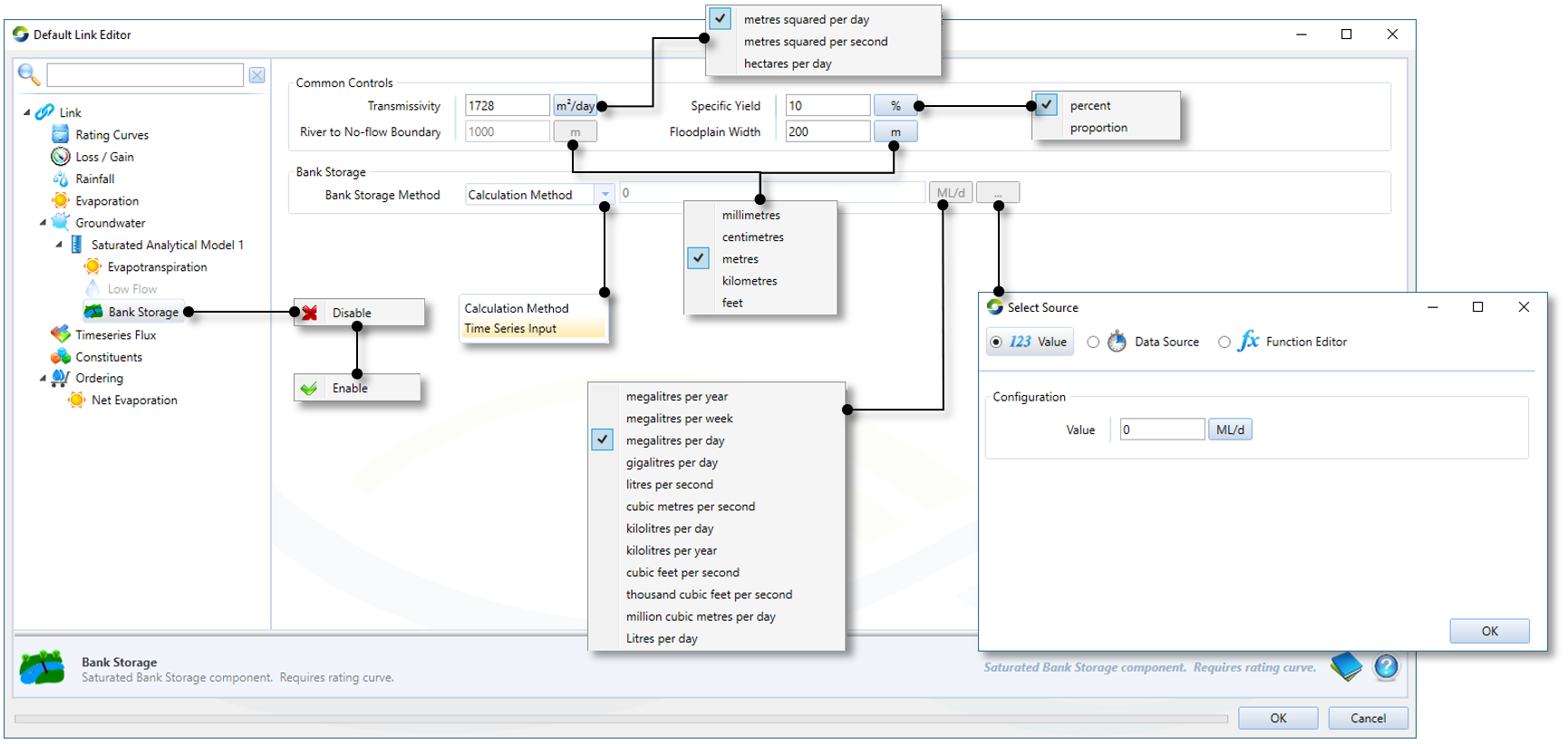
Bank Storage
There are two ways to generate a bank storage:
- Calculation method - this calculates the bank storage flux at run time from shared aquifer parameters and stream flow. At each time-step, the model takes the current stage height for the stream, the previous stage height for the stream, the floodplain width, aquifer transmissivity and aquifer diffusivity, and calculates a bank storage flux; or
- Load a known time series of bank storage fluxes. At each time-step, the model will retrieve a bank storage flux value and add it to the total groundwater flux generated for other saturated connection model processes under flooding conditions.
Figure 7. Groundwater, saturated (bank storage)
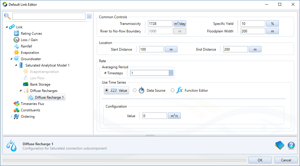
Diffuse recharge
Diffuse recharge (Figure 8) is a distributed source applied across a specified region within the floodplain. It infiltrates through the surface soil and recharges the aquifer, and if sufficient head difference is achieved, causes the aquifer to discharge water to the stream. The process model requires three shared aquifer parameters (Transmissivity, Specific yield and Floodplain width) and the following unshared parameters for:
- Location (start and end distances) - these refer to the closest and furthest orthogonal distances respectively from the river over which the recharge applies; and
- Recharge rate, specified as either a single value, a data source, or as a function. The units of the rate are entered as length2/time so that it is independent of the distance along the link that it is applied. It can be calculated as the volumetric rate divided by the length parallel to the river.
Figure 8. Groundwater, saturated (diffuse recharge)
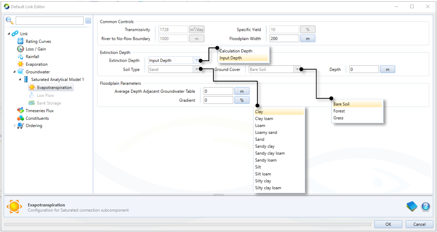
Evapotranspiration
The Evapotranspiration process model (Figure 9) calculates the amount of water which is lost from the aquifer by evapotranspiration (ie. plant transpiration and/or bare soil evaporation). The model requires Floodplain Width as a shared aquifer parameter and three process specific unshared parameters:
- Extinction Depth - the depth to water table at which ET no longer happens;
- Average Depth of Adjacent Groundwater Table - the average depth of the water table; and
- Gradient - the hydraulic gradient of the aquifer as a percentage.
Groundwater evapotranspiration is assumed to decrease with increasing depth to water table. The extinction depth is the depth at which groundwater evapotranspiration attains a value of zero.
Figure 9. Link (Groundwater, saturated, ET)
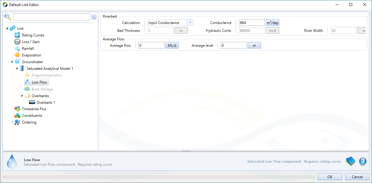
Low flow
A river may continuously lose water to, or gain water from the nearby aquifer; neutral cases are also a possibility (no head gradient with zero exchange). Consider a whole river-aquifer system that is at a steady-state, this exchange flux (gain or loss) would remain constant with time. It is given by:
DhxC
M
Where, Dh is the head difference, C is the hydraulic conductance of the river-aquifer interconnection and M is the thickness of river bed sediments.
Figure 10 shows the following unshared parameters to configure for low flow:
- Average flow - average river flow during low flow conditions; and
- Average level - average groundwater level during low flow conditions.
Figure 10. Groundwater, saturated (Low flow)
Overbank
Overbank (Figure 11) occurs when the stream stage height exceeds the height of the stream bank. Water flows over the stream bank and out onto the adjacent floodplain filling up any depressions and channels and creating inundated floodplain areas. The water in the inundated floodplain areas either evaporates or infiltrates through the soil and finds its way back to the stream. At each time-step, the model determines:
- Whether an overbank event has occurred;
- How much water is in any of the inundated floodplain areas;
- How much of this water is lost to evaporation; and
- How much water is returned to the stream (as a groundwater flux).
Figure 11. Groundwater, saturated (Overbank)
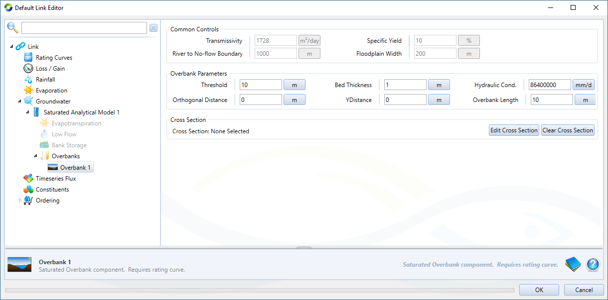
For each inundated floodplain area that you wish to model, an additional six parameters are required (outlined in Table 1).
Table 2. Saturated connection, Overbank parameters
| Parameter | Description |
|---|---|
| Bed thickness | The surface soil depth of the area. |
| Hydraulic conductivity | The hydraulic conductivity of the surface soil in the area. |
| Orthogonal distance | The orthogonal distance from the area centroid to the stream. |
| Overbank length | The length of the overbank feature parallel to the stream. |
| Threshold | A (unique) height (in mAHD) that river stage height must exceed to increase the area’s water volume. |
| YDistance | The distance from the area centroid to a line perpendicular to the stream through the upstream node (not currently used by the model but included for completeness). |
Additionally, you must specify the overbank feature's cross section using the Cross Section Editor.
Point recharge
Point recharge (Figure 12) works in a similar way as pumping from an unconfined aquifer except that, when recharge occurs, the cone of depression is inverted to form a groundwater mound, recharging the aquifer. If a sufficient groundwater head is developed the recharge water returns to the stream via aquifer discharge.
Since it is modelled in the same manner as pumping from an unconfined aquifer, they share similar parameters and the controls for entering these parameters are almost identical.
Figure 12. Groundwater, saturated (point recharge)

Table 3. Point recharge
| Parameter | Definition |
|---|---|
| Averaging period | The number of time-steps the timeseries will be averaged over. This is a tool to reduce computation time. Note that the timseries will be averaged for the specified number of timesteps and then applied to the following same number of time-steps. |
| Rate | Rate of pumping. This can be specified as a time series (as a single value, a data source or a function) or in terms of an account. |
Pumping
Groundwater pumping is one of the most important processes that impacts the exchange flux between groundwater and surface water. Pumping-induced river depletion is defined as the reduction of river flow due to induced infiltration of stream water into the aquifer or the capture of aquifer discharge to the river. As the cone of depression reaches the river, groundwater discharge to the river gradually reduces; when the cone of depression reaches the river, groundwater discharge to the river ceases. River water may eventually start infiltrating into the aquifer, contributing to groundwater pumping and thus marking the start of river depletion.
After a long period of pumping, the cone of depression takes its final shape (ie. a steady-state is reached), and a portion, or in some cases, all of the pumping will be balanced by a reduction in, or reversal of flow, from the aquifer to the river. The proportion of pumping met by river depletion in the steady-state case will depend on various factors, including the proximity of the bore to the river compared to the distance between the bore and other stresses to the groundwater system (eg recharge, ET).
Source allows for two types of groundwater pumping:
- Pumping from an unconfined aquifer (Figure 13) with or without a no-flow boundary - This caters for pumps which tap directly into an aquifer (with or without a no-flow boundary) which is hydraulically connected to the stream. The pump is at a given distance from the stream, it switches on at some time, pumps at a constant rate for a period (the pumping period may occur prior to the simulation start time and the effects are still modelled) and then switches off; and
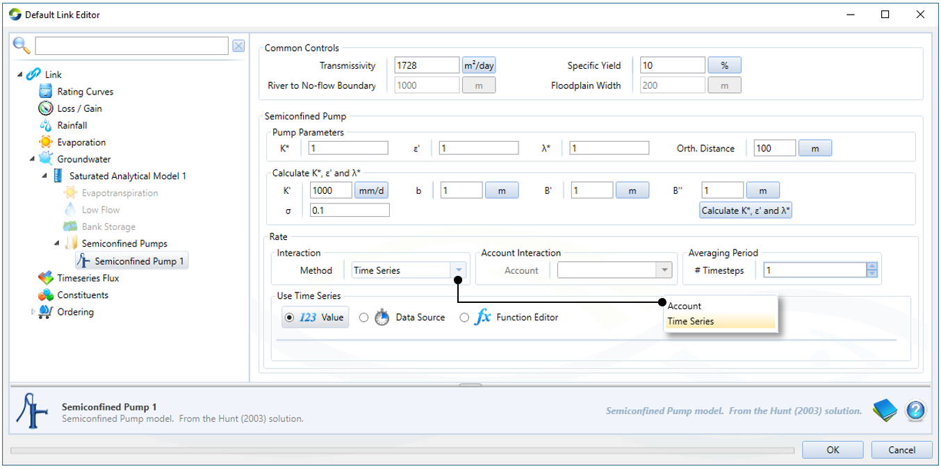
- Pumping from a semi-confined aquifer (Figure 14) - used to model pumps which tap into a semi-confined aquifer which is hydraulically connected to the stream. Again, the pump is either connected to an account for a Water User or specified as a timeseries of pumping rate.
You could enter the parameters for each process, or import a .csv file containing this information.
Table 3 contains parameter definitions for Figure 13. Note that some parameters have been defined in Table 1.
Figure 13. Groundwater, saturated (Unconfined pumping)
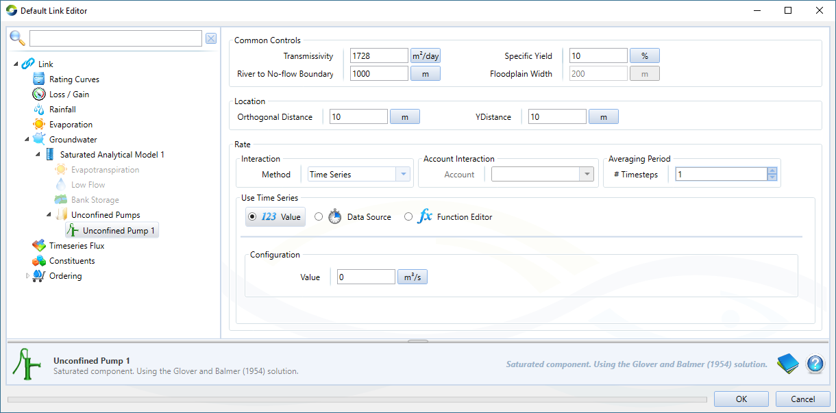
Table 4 outlines the parameters under Semiconfined Pump of Figure 14.
Table 4. Groundwater pumping, semi-confined
| Parameter | Definition |
|---|---|
| Orth. distance | The orthogonal distance between the river and the pump. |
| b | Nominal stream width. |
| B' | Aquitard saturated thickness. |
| B'' | Aquitard thickness beneath stream. |
| epsilon | Non-dimensional variables used in the Hunt (2003) equation. |
| lambda | Streambed resistance coefficient. |
| K' | Aquitard permeability. |
| K* | Non-dimensional variables used in the Hunt (2003) equation. |
| sigma | Aquitard porosity. |
Figure 14. Groundwater, saturated (semi-confined)