Note: This is documentation for version 4.11 of Source. For a different version of Source, select the relevant space by using the Spaces menu in the toolbar above
Multi-objective optimisation - Insight - SRG
Overview
Description and rationale
Insight is eWater’s multiple-objective optimisation and decision support framework. This framework allows for more efficient evaluation of planning options than the traditional manual trial and error approach that modellers often use. The optimisation tool enables a more thorough examination of potential planning scenarios and the resulting trade-offs between desired outcomes.
Insight allows the modeller to define which parameters are to be considered in the optimisation framework. These parameters are called "decision variables". For example, the requirement might be to develop operating rules for a new desalination plant that meet the objective of minimising cost, or to identify what the optimal operating rules are for transferring water between storages to meet supply security objectives and minimising environmental impacts. By creating decision variables for these operating rules, the optimiser will try hundreds or thousands of different operating rules based on the chosen decision variables and determine how the rules perform against a set of user-specified objectives.
Insight links a multi-objective optimiser (Deb et al., 2002) to Source’s external interface and optimises Source models by running them many times with different parameter values.
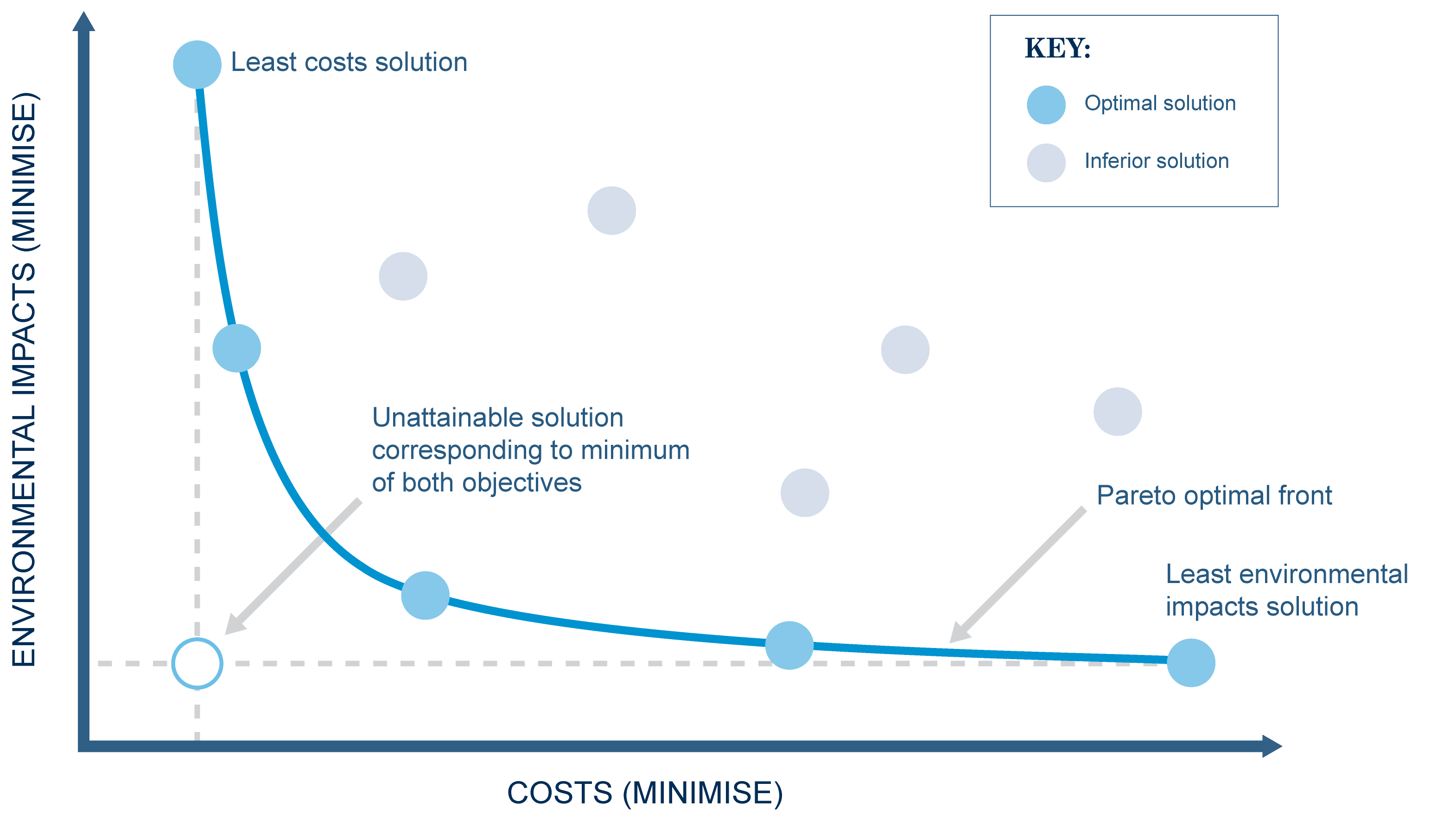
For example, if the requirement is to minimise both costs and adverse environmental impacts, then Insight will search for options which express the trade-offs between these two competing objectives. Each solution has different cost and performance outcomes. Insight does not make any judgements about how important each of the impact statistics are, instead it searches a range of options which have different types of impacts. Insight will only discard an option, ‘A’, if it is clearly inferior to an alternative option, ‘B’. That is, if ‘B’ performs better than ‘A’ on at least one of the statistics and there is no statistic where ‘A’ performs better than ‘B’. At the end of its run, Insight will produce a range of optimal solutions (the Pareto Front). Figure 1 shows an example (after Blackmore et al., 2009).
The optimisation results can be examined via a number of graphical tools to help the planners consider the trade-offs between objectives and the relationship between decisions and objectives.
Figure 1. Example Pareto Front diagram (after Blackmore et al., 2009)
Insight operates at the spatial and temporal scales of Source models. It runs Source models multiple times to search for optimal solutions.
Principal developer
The multi-objective optimiser used in Insight was developed by Deb et al. (2002). It was originally adapted for use with Source by eWater CRC with permission.
Insight was originally developed by eWater CRC and has subsequently been enhanced by eWater Ltd to meet the needs of the Melbourne Water Corporation.
Scientific Provenance
The multi-objective optimiser used in Insight is the Non-dominated Sorting Genetic Algorithm II (NSGA-II) developed by Deb et al. (2002). This is a Multi-Objective Evolutionary Algorithm (MOEA) that is based on the principles of the well known Genetic Algorithm (GA).
Version
Source v3.8.8.
Dependencies
Insight requires a functioning Source model to work with.
Availability/conditions
Use this heading if the functionality is a plugin or requires any 3rd party software applications.
Structure & processes
Theory of NSGA-II
Details of the derivation of the Non-dominated Sorting Genetic Algorithm II (NSGA-II), including pseudo-code, are available in Deb et al. (2002). NSGA-II is a variant of the well known Genetic Algorithm (GA) and the principles of the GA are discussed in text books (e.g. Loucks and van Beek, 2005).
Key features of NSGA-II are (abridged from Deb et al., 2002):
- A fast non-dominated sorting approach. This is used to find population members in the best, second best, third best, etc., non-domination levels.
- Diversity preservation based on a crowded distance estimation procedure and a crowded comparison operator. This approach does not require any user-defined parameter for maintaining diversity among population members.
A computational algorithm summarised as follows:
Initially create a random parent population, P1 of size N and sort this population using the fast non-dominated sorting approach.
Use binary tournament selection, recombination (crossover) and mutation operators, to create the first offspring population, Q1, of size N.
Noting that elitism is introduced by comparing the current population with previously found non-dominated solutions then the procedure after the initial generation can be summarised by considering the i’th generation:
- Create a combined population Ri = Pi U Qi, where Ri has size 2N, and sort this combined population using the fast non-dominated sorting approach.
- Start assembling a new population Pi+1 of size N. The assembly process begins by including solutions at the best non-dominated level. If the number of these is less than N then they are all included. This process continues with solutions from the second best, etc. levels as long as all the solutions from these levels can be included (i.e. the combined total of these solutions is less than N). For the last level (i.e. the one where not all solutions can be included to make up the numbers to N), the solutions are sorted using the crowded comparison operator to identify the best ones to include in the new population.
- The new population Pi+1 is used for selection, crossover and mutation to create a new offspring population Qi+1 of size N. For selection a binary tournament selection operator is used but the selection criterion is now based on the crowded comparison operator.
Definitions
| Decision variables | The management levers which can be pulled in order to achieve the required objectives. Each decision variable must be defined as a global Function, with an allowable range of values it can take. |
| Dominated solution | When comparing results from two Source runs (or group of runs), ‘A’ and ‘B’, Insight will treat ‘A’ as a “dominated solution” only if it is clearly inferior to ‘B’; that is, if ‘B’ performs better than ‘A’ on at least one of the statistics and there is no statistic where ‘A’ performs better than ‘B’. In this case ‘B’ is a “non-dominated solution” and is a potential candidate for the Pareto front of optimal solutions (e.g. see Figure 1). |
| Generation | For each generation the decision variables are subject to selection, crossover and mutation. The number of generations is specified by the modeller. |
| Individual | A solution obtained from a single run of Source with a given set of decision variable values (an individual is a group of runs when multiple scenarios are being investigated: one run for each scenario). |
| Non-dominated solution | See definition of “dominated solution”. |
| Objective function | Mathematical expression of the objectives required to be achieved (e.g. minimising the operating cost of the system, maximising environmental benefits, or minimising time spent in water restrictions). Objective Functions are set up as global Functions within Source. Note that only the value of the Function at the last time step is used for evaluating the objective function. Therefore, Function should be defined in such a way that the value at the last time step of the simulation is the value that represents the required statistic for the entire simulation period. |
| Population | The number of possible feasible solutions to be derived by changing decision variable values (within their value constraints) in Insight and running Source. The population size is specified by the modeller and is equal to the total number of individuals. |
Insight Functionality
User requirements are summarised in Table 1. Interactions between Insight and Source are shown in Figure 2.
Table 1. User requirements
| Item number | Prioirity | Short description of task |
|---|---|---|
| 1 | 1 | Allow optimisation over multiple scenarios |
| 2 | 4 | Suitable output for multi-replicate runs |
| 3 | 4 | A tool for analysing results from multi-replicate output |
| 4 | 6 | Allow sub-models of Source with different time steps |
| 5 | 5 | User-customisable water balance report |
| 6 | 1 | Allow objective functions to be a range of statistics |
| 7 | 3 | Insight to report the values of secondary objective functions |
| 8 | 2 | Pass user-selected decision variables from Insight to Source |
| 9 | 7 | Implement climate/component flexible restriction modelling |
| 10 | 8 | Allow 2-way flow |
| 11 | 9 | Implement sub-networks |
| 12 | 10 | Link models with different time steps, e.g. Urban Developer |
| 13 | 11 | Enable switching between rules-based and NetLP |
| 14 | 12 | Recycling of n years of historical data |
A single scenario in a Source model could represent a particular system configuration, inflow sequence, demand model, etc. Insight can optimise the decision variable(s) (DVs) over multiple scenarios. The DVs and objective functions are chosen by the modeller.
Figure 2: Flowchart of interactions between Insight and Source for multi-scenario optimisation
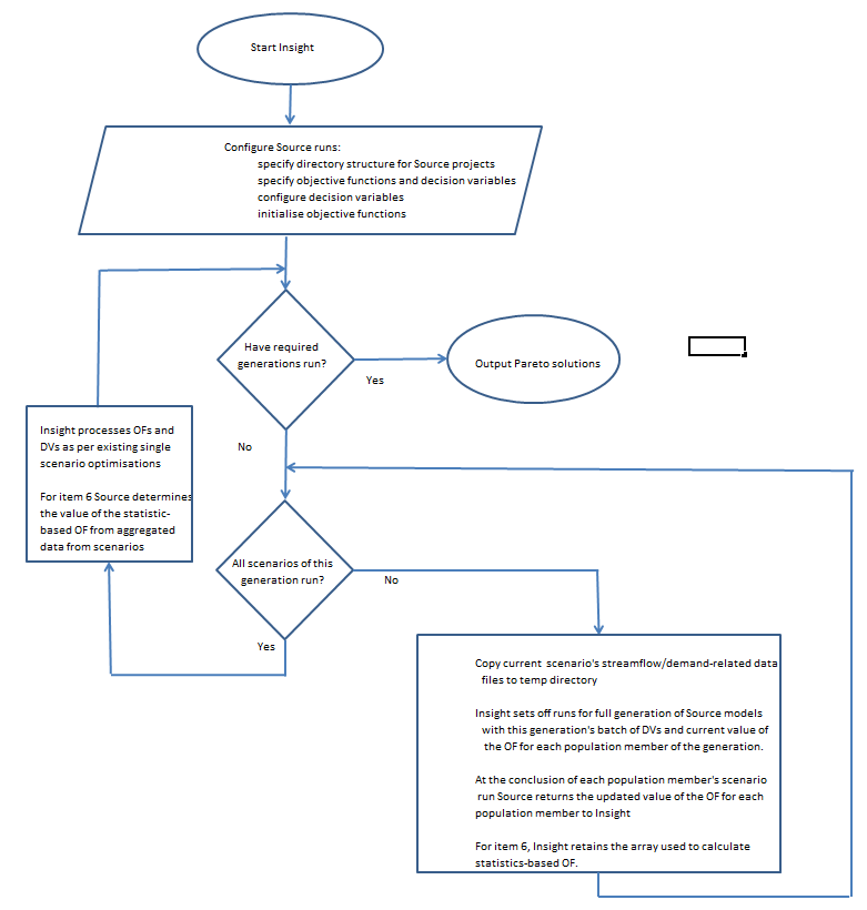
Key features are:
- The same set of DVs applies to all scenarios for each run of a batch of scenarios
- The values of the OF(s) are aggregated for each population member for all scenarios in a run of a batch of scenarios
- Statistics-based OFs are determined within Insight.
The functionality listed in Table 1 is all concerned with input and output data handling and how Insight and Source interact, and there is no new science involved. Therefore, the functionality in Insight is not discussed further here and reference should be made to the Insight: Multi-objective optimisation for information on how to use it.
Process
(Also refer to Figure 2)
1st generation
- Values of decision variables, randomly chosen by Insight from within their allowable value ranges (where these ranges are input by the modeller), are passed to Source (Step 3(a) in the section on Theory of NSGA-II). Insight provides one set of values for every “individual”, where the number of individuals is equal to the population size input by the modeller.
- Source is run for each individual (this is a group of runs for each individual when multiple scenarios are being investigated: one for each scenario).
- Values of objective functions and result variables needed for evaluating statistical objective functions are passed back from each run of Source to Insight.
- New values of decision variables are derived by selection, crossover and mutation to create the first offspring population (Step 3(b) in the section on Theory of NSGA-II).
- Source is run for each individual in this population (group of runs when multiple scenarios are being investigated).
- Values of objective functions and result variables needed for evaluating statistical objective functions are passed back from Source to Insight at the end of the run(s) for each individual.
Subsequent generations
For the i’th generation where 1 ≤ i ≤ ng (and the total number of generations, ng, is input by the modeller):
- Insight processes decision variables and objective functions using the procedure described in the first two bullet points in Step 3(c) in the section on Theory of NSGA-II to create a new population (Pi+1). When comparing results from two Source runs (or group of runs), ‘A’ and ‘B’, Insight will treat ‘A’ as a “dominated solution” only if it is clearly inferior to ‘B’; that is, if ‘B’ performs better than ‘A’ on at least one of the statistics and there is no statistic where ‘A’ performs better than ‘B’. In this case ‘B’ is a “non-dominated solution” and is a potential candidate for the Pareto front of optimal solutions (e.g. see Figure 1).
- Values of each decision variable from the new population (Pi+1) are used for selection, crossover and mutation by Insight (i.e. the third bullet point in Step 3(c) in the section on Theory of NSGA-II) to create a new offspring population (Qi+1) of decision variables. The resultant values of decision variables are passed to Source.
- Source is run for each individual (or group of runs when multiple scenarios are being investigated).
- Values of objective functions and result variables needed for evaluating statistical objective functions are passed back from Source to Insight at the end of the run(s) for each individual.
- Insight processes decision variables and objective functions from the current and previous generations (i.e. repeats Step 1 above), searching for “dominated solutions” and “non-dominated solutions”.
- If all generations have been run, the resultant set of “non-dominated solutions” is the final set and is the Pareto front of optimal solutions. Otherwise the process repeats Steps 2-5 above.
Data
Input data
At a minimum, Insight requires the following information to run an optimisation:
- One or more Source scenarios containing decision variables and objective functions
- Access to the Source command line tool
- An Insight settings file (containing the Source project location, objective functions and decision variables)
- The number of generations
- The population size of each generation
The decision variables and objective functions must be defined in the Source project as global Functions. Hence, in order for a Source parameter to be included in an optimisation problem, that parameter needs to be able to be defined through the Function editor.
More details on data are provided in the Source User Guide.
Parameters
| Parameter | Description | Units | Default | Range |
|---|---|---|---|---|
| Population (N) | Number of individuals (i.e. sample size) in each generation. | none | none | Should be sufficiently large to enable statistically meaningful results to be obtained (e.g. 8 ≤ N ) but not so large that the additional samples contribute very little to finding the optimal solution set. |
| Generations (ng) | Governs the number of times decision variables are to be subject to selection, crossover and mutation processes. | none | none | 1 < ng but ng should not be so large that the later generations contribute very little to finding the optimal solution set. |
Output data
Outputs include values of decision variables and objective functions for each individual for each generation, to enable viewing in graphical displays and tables and further processing. The graphical displays include a plot that is updated after each individual is run in Source which shows the progressive development of the Pareto Front.
Once more than one generation is complete Insight allows for the hypervolume (Emmerich et al, 2005; Fonseca et al, 2006; Knowles et al, 2006) to be viewed. This provides an indication of how the results are converging towards the Pareto optimal solution. The hypervolume is calculated based on the distance between a maximum non-optimal solution and the modelled results, and the larger the hypervolume, the closer the results are to reaching the Pareto optimal solution. Graphing this provides a useful indication of how much the optimal solutions are changing. If the hypervolume plot is flattening out then this is an indication that more generations are unlikely to produce better results.
All items selected for recording in the Source Recording Manager by the modeller from single and multi-replicate model runs are written to file by Source so that results are able to be analysed for selected outputs:
- For all replicates
- For any selected replicate
- Statistics across all replicates
The structure of the file is:
Rows 1 – 5 Header lines with run and output information. These are used to record metadata such as project file name and description, scenario name and description, user name, run date and time, initial storage volumes (to be used for item 5 – water balance report) etc.
Row 6 – Fortran free format statement for time series data in the file (i.e. *).
Row 7 – number of columns of data inclusive of date and replicate number (ncol)
Row 8 – 8 + ncol - 1 – descriptors for each column
Subsequent rows – time series data of the following form:
Timestep 1, replicate 1 season, year, replicate, requested outputs
Timestep 2, replicate 1 season, year, replicate, requested outputs
Timestep 3, replicate 1 season, year, replicate, requested outputs
Tiimestep …, replicate 1 season, year, replicate, requested outputs
Timestep 1, replicate 2 season, year, replicate, requested outputs
Timestep 2, replicate 2 season, year, replicate, requested outputs
Timestep 3, replicate 3 season, year, replicate, requested outputs
Tiimestep …, replicate 4 season, year, replicate, requested outputs
… and so on.
A separate stand-alone tool is available that produces the following statistics and output for modeller selected items or all items in the above file:
- For all replicates, or for a selected replicate, with a user-definable year (only full years considered)
- Overall maximum
- Mean and standard deviation of annual maximums for all/selected replicate(s)
- Specified percentile of annual maximums for all/selected replicate(s)
- Overall minimum
- Mean and standard deviation of annual minimums for all/selected replicate(s)
- Specified percentile of annual minimums for all/selected replicate(s)
- Mean and standard deviation of value for all/selected replicate(s)
- Items I – VII for a specified annual date
- Items I – VI for accumulated values for a specified annual date range
- Export to a separate file modeller selected time series selected by replicate number and/or item. This file has same format as above.
Reference list
Blackmore, J. M., Dandy, G. C., Kuczera, G. and Rahman, J. (2009). Making the most of modelling: a decision framework for the water industry. In 18th World IMACS / MODSIM International Congress on Modelling and Simulation, edited by R. S. Anderssen, et al. Cairns, Australia: Modelling and Simulation Society of Australia and New Zealand and International Association for Mathematics and Computers in Simulation.
Deb, K., Pratap, A., Agarwal, S. and Meyarivan, T. (2002). A fast and elitist multiobjective genetic algorithm: NSGA-II. IEEE Transactions on Evolutionary Computation, 6(2): 182-197.
Emmerich, M., Beume, N. and Naujoks, B. (2005). An EMO algorithm using the Hypervolume measure as selection criterion. Carlos A. Coello Coello, Arturo Hernández Aguirre, Eckart Zitzler (Eds): Evolutionary Multi-Criterion Optimization, Third International Conference, EMO 2005, Guanajuato, Mexico, March 9-11, 2005. Proceedings. Lecture Notes in Computation Science, 3410: 62-76.
Fonseca, C.M., Paquete, L. and López-Ibáñez, M. (2006). An improved dimension-sweep algorithm for the Hypervolume indicator. Proceedings of the IEEE Congress on Evolutionary Computation, Vancouver, Canada, July 16-21, 2006. 1157-1163.
Knowles, J.D., Thiele, L. and Zitzler, E. (2006). A Tutorial on the Performance Assessment of Stochastic Multiobjective Optimisers, TIK Report Number 214, ETH Zurich.
Loucks, D.P. and van Beek, E. (2005). Water resources systems planning and management: an introduction to methods, models and applications. UNESCO, Paris and WL | Delft Hydraulics, The Netherlands. 680 pp. ISBN 92-3-103998-9. Available at: ecommons.library.cornell.edu/handle/1813/2799.