Note: This is documentation for version 4.11 of Source. For a different version of Source, select the relevant space by using the Spaces menu in the toolbar above
NetLP - SRG
During each time-step, Source operates in two phases: the ordering phase and the flow distribution phase. The ordering phase accumulates orders and determines the targets for release and distribution of regulated water. The flow distribution phase releases water, routes flows and distributes water through the river network.
During the ordering phase, the release of water to satisfy orders can be computed in one of two ways:
- statically, using a set of predefined rules, or
- dynamically, using a Network Linear Program (NetLP) to find an optimal solution.
Source refers to the latter as Optimised Ordering.
Why use Optimised Ordering?
It is often desirable to operate multiple storages in such a way as to maintain pre-determined relationships between them. Scenarios include:
- storages in series on the same branch of a river system;
- storages located in different branches of a river system and operated in parallel; or
- combinations of both of the above.
It is also possible to have multiple paths for the transmission of water, such as occur in the presence of anabranches.
Determining optimum release and travel patterns is complex and the network linear program employed by Optimised Ordering can assist operators in making decisions to run a river system efficiently.
Scale
One or more iterations per time-step.
Principal developer
RELAX IV was developed by Dimitri Bertsekas, and some bindings to RELAX IV were developed by George Kuczera. PPRN was developed by Jordi Castro. The implementation of these in Source is specific to eWater CRC.
Version
Source version 3.0.2
Availability/conditions
Version 1 of Source will not include performance tuning for runtimes, full side constraint capability, complex ownership interactions, routing, or partial optimisation.
Theory
The standard form of a linear programming function is as follows:
| Equation 1 | 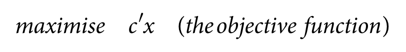 |
|---|
subject to the constraints:
| Equation 2 | 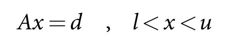 |
|---|
where:
x represents the vector of variables to be determined
c is an n-vector of costs or penalties
d is an m-vector of known nodal inflow or outlow volumes (coefficients)
l and u are lower and upper bounds, respectively, on x
A is a (m,n) node-incidence matrix of whose (i,j)th element is defined:
Equation 3 | if arcjis directed towards nodei | |
|---|---|---|
| otherwise | ||
| if arcjis directed away from nodei |
The constraint AX=d ensures that mass balance is achieved at every node in the network. This is always the linear program solver’s highest priority.
Optimisation (Linear programming) algorithms
Source currently supports the following optimisation algorithms:
- PPRN with side constraints
- PPRN without side constraints
- PPRN with network duplication
- RELAX IV
- RELAX IV with network duplication
PPRN uses real numbers and is a true linear programming algorithm. RELAX IV uses integers and is more properly described as an integer programming algorithm.
Side constraints
Side constraints are implemented, automatically, by translating between requirements set in nodes or links in the Source schematic, to constraints imposed on the arc-node model provided to the solver.
Side constraints can enforce requirements and can also promote more rapid convergence by eliminating options.
Only PPRN supports side constraints.
Assumptions
All linear programs assume perfect data. To the extent that the data provided to the solver by Source does not satisfy this assumption, the solutions found by the solver may be sub-optimal.
Source integration
The details of the operation of the network linear program are largely hidden from the user. Source performs the translation between the per-scenario Node-Link network visible in the Schematic Editor and the arc-node network which is created for each time-step for use by the network linear program. Source also manages the numbers of iterations which are required at each time-step. Figure 1 summarises how Source interacts with the network linear program.
Notes:
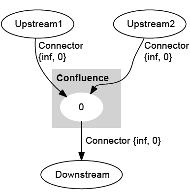
Inflow forecasting: In general, inflow forecasting for NetLP works in the same way as it does for Rules Based Ordering (see the Rules-Based Ordering - SRG entry for details). A point to note is that NetLP models are often monthly. In monthly models, the basis for inflow forecasts at inflow nodes and unregulated confluences often differs from that for shorter time step models such as daily models. In a daily model the forecast for each time step's inflow is typically based on a recession from the previous time step's inflow. In a monthly model the forecast inflow is typically the actual inflow for the time step. To achieve this the Trend Forecast Model is configured with a (recession) rate of 0.0, and there is no forecasting from the current time step.
Travel times: In the order phase for NetLP, travel time is modelled by making a replica of the appropriate parts of the network for each full time step's travel time (up to the maximum network travel time) and aggregating into a single network. The aggregated network is then solved, giving a solution as far forward as the maximum network travel time. This allows optimised orders to be determined the appropriate time in advance (note that NetLP models are often monthly and, as travel times used for ordering are rarely, if ever, longer than this, for monthly models only the current time step is considered). The orders are then passed to the flow phase where processing occurs as per rules based ordering (see the Rules-Based Ordering - SRG entry for more information).
Figure 1. Source - NetLP interaction
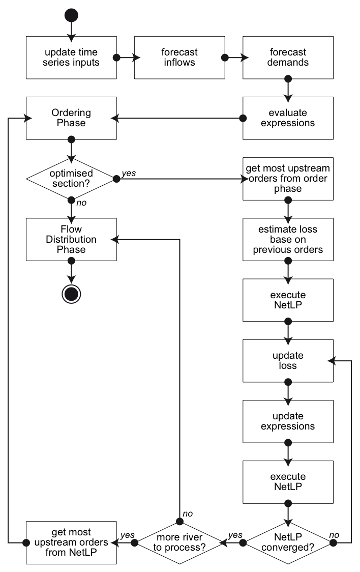
In each time-step, the NetLP needs to solve an arc-node network to determine a set of releases for a given set of orders and constraints.
Where capacities and demands vary according to predicted flows, the NetLP needs to arrive at a solution iteratively. An optimised solution is considered to have been found when the differences between two successive iterations fall within specified limits.
The optimised solution provides the flow distribution phase with order information for that time-step, including the best way to supply the orders and to move water through the system.
The flows observed during the flow distribution phase will generally be greater than or equal to the ordered flows unless, for example, losses were greater than estimated, or actual inflows less than those originally forecast.
Arc-node translation
This section contains a selection of arc-node models which are typical of those generated by Source. The information presented here can not possibly cover all possible permutations and combinations. As a result, it should be considered broadly informative without being necessarily either comprehensive or authoritative.
Each arc connecting two nodes within a model carries an annotation of the form shown in Figure 2:
Figure 2. Arc definition

Arcs are uni-directional with arrow-heads indicating the direction of flow. In addition:
- An arc with a zero cost represents neither an incentive nor a disincentive.
- An arc with a positive cost has a cost disincentive. The greater the magnitude of the positive number, the greater the disincentive for water to flow along that arc.
- An arc with a negative cost represents a cost incentive. The greater the magnitude of the negative number, the greater the incentive for water to flow along that arc.
The default costs for arcs are predefined within Source.
Ownership is modelled by constructing replicas of the system for each owner, containing only those features to which the owner has access.
Replicas are also used to model transmission delays in the system.
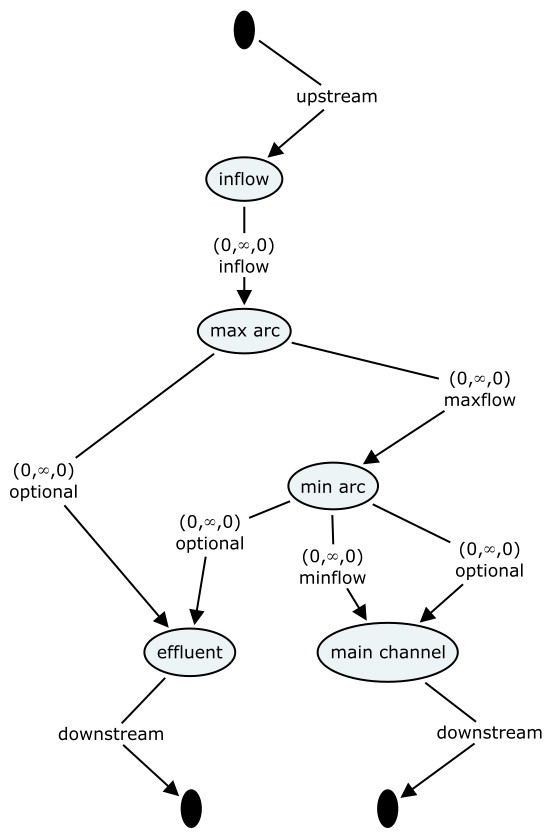
Splitter
A splitter (regulated or natural system) forces the proportion of water allocated to the effluent to flow down that path, with the balance travelling down the main channel. The proportion of water allocated to the effluent (or regulated side) is set in the Splitter (or Regulated Splitter) node using a piecewise linear editor. See Figure 3.
Figure 3. Arc-node diagram, Splitter
Minimum Flow Requirement
A minimum flow requirement is implemented by a two-arc construct. The requirement has a high incentive arc limited to the value of the constraint. Any water beyond the minimum will flow via the excess path which has a zero cost. The constraint is set on the corresponding Minimum Flow Requirement node in the Source schematic. See Figure 4.
Figure 4. Arc-node diagram, Minimum Flow Requirement
Maximum Order Constraint
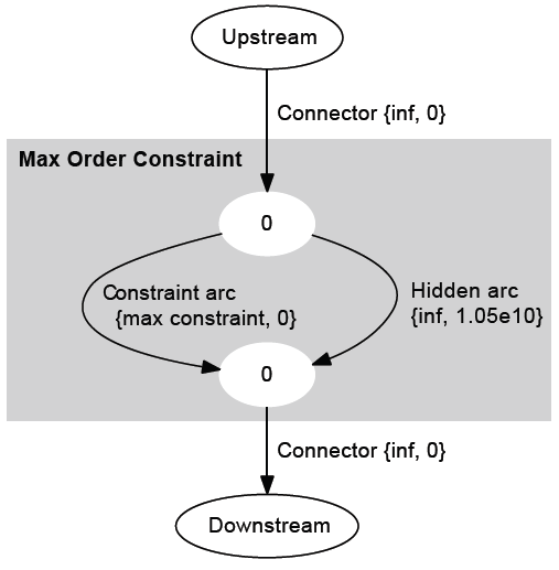
A maximum order constraint is implemented by a two-arc construct. The constraint has a zero cost arc limited to the value of the constraint. Any water beyond the maximum may flow via the hidden path which has a very high disincentive. In effect, any water over and above the constraint equates to a flood condition. The constraint is set on the corresponding Maximum Order Constraint node in the Source schematic. See Figure 5.
Figure 5. Arc-node diagram, Maximum Order Constraint
Loss
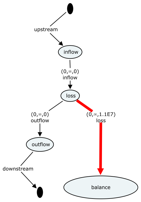
A loss forces the proportion of water lost from the system to flow to the balance node over a high-incentive arc. The proportion of loss is set on the corresponding Loss node in the Source schematic using a piecewise linear editor. See Figure 6.
Figure 6. Arc-node diagram, Loss
Supply Point
A demand draws an amount of water via an extraction point node. Demands are created using the various kinds of Water User node within the Source schematic. If there is sufficient water in the system to satisfy a given demand, the volume required flows to the extraction point node with any excess returned to the balance node. If there is insufficient water in the system to satisfy demand, any shortfall may be satisfied via the shortfall arcs running between the balance node and the extraction point node, according to the extraction point node’s priority, relative to other extraction point nodes in the system. See Figure 7.
Figure 7. Arc-node diagram, Supply Point and Water User
.png?version=1&modificationDate=1349336679517&cacheVersion=1&api=v2&width=800&height=233)
Storage
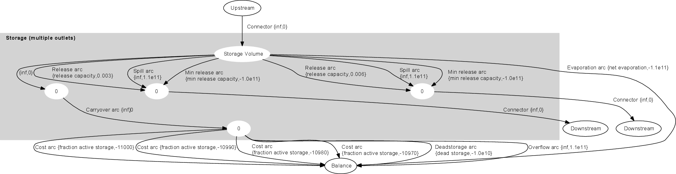
Within a storage, evaporation is satisfied first. This is implemented as a very-high-incentive arc to the balance node. There is an incentive to retain water in storage. This is achieved via the storage carry-over arcs which convey most of the stored water in a time-step to the balance node, where it carries-over to the next time-step. The number, priorities and volumes of the carry-over arcs (break-points) for a given storage can be set relative to other storages in the system to implement various release and operational objectives. See Figures 8 and 9.
Figure 8. Arc-node diagram, Storage
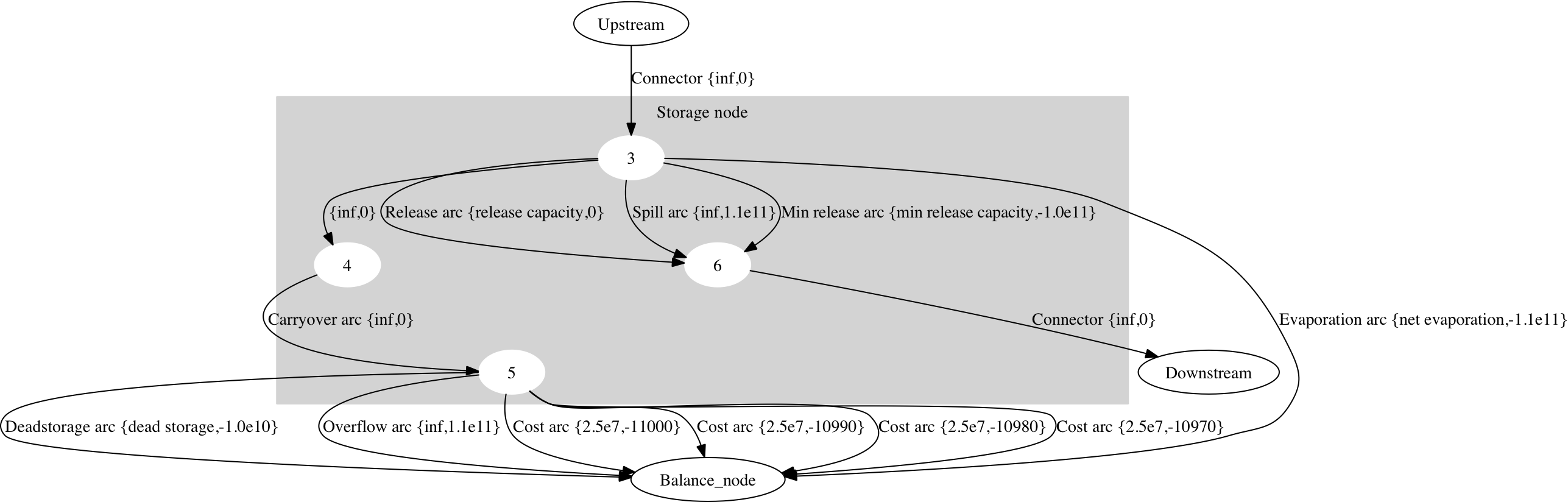
Figure 9. Arc-node diagram, Storage (multiple outlets)
Input data
All data is supplied to the solver automatically by Source. There are no separate or externally-configurable data sources.
Solvers use arc-node networks as their inputs. Source derives arc-node networks automatically for each time-step from the node-link network in the Schematic Editor.
Source provides information from the previous flow phase at the start of each time-step to initialise the NetLP, such as storage volume in reaches and reservoirs, water use requirements, forecast inflows and current ownership of water in storages and reaches.
Source uses real numbers internally. When RELAX IV is chosen as the optimisation algorithm, all real numbers are scaled on entry to, and on return from, RELAX IV, to minimise loss of precision.
Output data
The solver provides the flow distribution phase with information on how to distribute flow at regulators, constraints on demands and ownership of orders at each storage and routing reach.
There may be differences between the solution found by the solver ("as predicted") and flows as modelled during the flow distribution phase ("as released"). The flow distribution phase resolves these differences by considering the ordering phase as having provided a minimum target to aim for.
Iteration control
The NetLP iterates to find the optimal solution. Usually, the NetLP will find a solution quickly. Under some circumstances, the NetLP will not converge upon a solution quickly and will keep iterating. The user can limit the number of iterations to force acceptance of a (possibly) sub-optimal solution. The user can also set tolerance thresholds to define per-arc convergence criteria.
Cost functions
Cost functions determine both the relative importance of keeping water in a storage, and the relative importance of water in one storage compared with water in another storage. By default:
Each storage has a single cost function comprising four break-points associated with 25% of the storage’s capacity.
All storages are considered equal, regardless of differences in capacity.
Cost functions have a granularity of one month (ie. while a given cost function can be applied to a storage for zero or more months, only one cost function can be applied to a storage for any given month).
Cost functions are designed using the Source user interface.
Shortfalls
A shortfall occurs when there is insufficient water in a system to satisfy all demands. Source provides a mechanism for instructing the solver how to prioritise competing demands.
Bibliography
Bertsekas, D.P. & Tseng, P. 1994, RELAX-IV: A faster version of the RELAX code for solving minimum cost flow problems, Technical Report P-2276, Massachusetts Institute of Technology, http://www.mit.edu/dimitrib/www/noc.htm [retrieved 11 March 2010].
Bertsekas, D.P. 1991, Linear network optimization: algorithms and codes, The MIT Press.
Castro, J. 1994, PPRN 1.0, User’s Guide, Statistics & Operations Research Dept, UPC, ftp://ftp-eio.upc.es/pub/onl/reports/dr1994-06.pdf [retrieved 11 March 2010].
Castro, J. & Nabona, N. 1996, "An implementation of linear and nonlinear multicommodity network flows", European Journal of Operational Research, vol. 92, no. 1, pp. 37-53.
Chen, J., Kim, S., Penton, D., Kinsman D. and Welsh, W. 2011, "Visualising Equivalent System Networks in the NetLP Optimisation of Water Distribution Systems", 19th International Congress on Modelling and Simulation, Perth, Australia, 12-16 December 2011, pp. 2303-2309.
Delgado, P., Kelley, P. Murray, N. & Satheesh, A., Source User Guide, eWater Cooperative Research Centre, Canberra, Australia.
Gilmore, R. 2009, River Systems Project : Source Rivers : Optimised Multiple Supply Modelling : Specification : Version 1.0, eWater Cooperative Research Centre, Canberra, Australia.
Gilmore, R.L., Kuczera, G., Penton, D. & Podger, G. 2009, "Improving the efficiency of delivering water in Australian river systems: modelling multiple paths", 18th World IMACS / MODSIM Congress, Cairns, Australia 13-17 July 2009, pp. 225-231.
Gilmore, R. 2008, Multiple Supply Paths Test Case: Lachlan River System, NSW, eWater Cooperative Research Centre, Australia.
Ilich, N. 2008, "Shortcomings of linear programming in optimizing river basin allocation", Water Resources Research, vol. 44, no. 2, pp. W02426.
Ilich, N. 2009, Limitations of etwork Flow Algorithms in River Basin Modeling, Journal of Water Resources Planning and Management, vol. 135, no.48, pp.1-8
Israel, M.S. & Lund,J.R.1999, Priority preserving unit penalties in network flow modeling, J. Water Resources Planning Manag., vol.125,no.4, pp. 205-214 Kuczera, G. 2008, Lag network diagrams (personal files), University of Newcastle, Callaghan, NSW.
Kuczera, G. 1989. "Fast multireservoir multiperiod linear programming models." Water Resour. Res., vol.25, no.2, pp.169-176
Kuczera, G. 1992, "Water supply headworks simulation using network linear programming", Advances in Engineering Software, vol. 14, no. 1, pp. 55-60.
Kuczera, G. & Diment, G. 1988, General water-supply system simulation model-WASP. J Water Resour Plan Manage-ASCE, vol.114,no.4, pp.365-382
Penton, D. 2009, Multiple Supply Path : Design Document : Optimisation, eWater Cooperative Research Centre, Canberra, Australia.
Penton, D. 2009, The NetLP Ordering Component : Guide and Introduction, eWater Cooperative Research Centre, Canberra, Australia.
Perera, B.J.C. & James, B. 2003, "A generalised water supply simulation computer software package-REALM", Hydrology Journal, Institute of Engineers, India, vol. 26, no. 1-2, pp. 67-83.