Note: This is documentation for version 4.11 of Source. For a different version of Source, select the relevant space by using the Spaces menu in the toolbar above
Rectangular Weir Calculations
Geometric notions
To perform the calculations necessary to describe and manage the flow in a weir, it is necessary to examine the geometry of the storage area created by the weir. This, in particular, allows us to determine the configuration of the weir when occupied by a specified volume of water, or conversely, when the volume of water in the weir pool is known, to determine the depth and weir extent.
For the purpose of the Weir model with rectangular geometry it is assumed that:
- The reach is of constant width in the neighborhood of the weir
- The river bed slopes downward at a constant angle θ to the horizontal
- The weir gates are lowered after the reach has been flowing with the gates raised
- Some of the water previously assumed to have been routed downstream will now be stored behind the weir, occupying a wedge-shaped region.
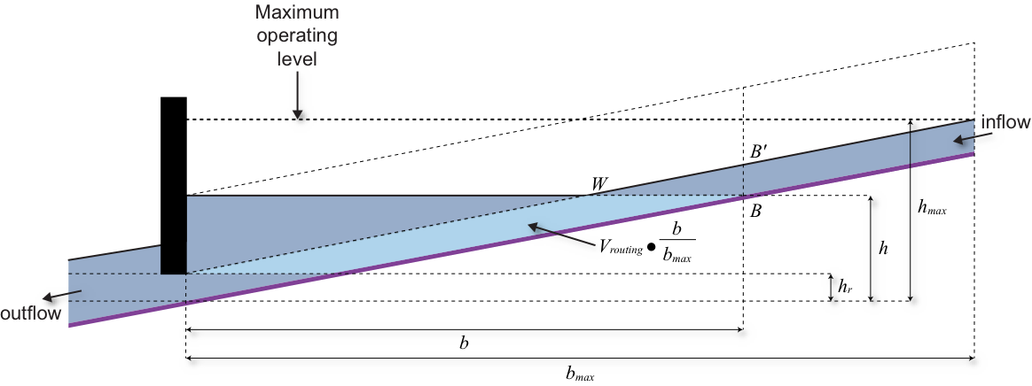
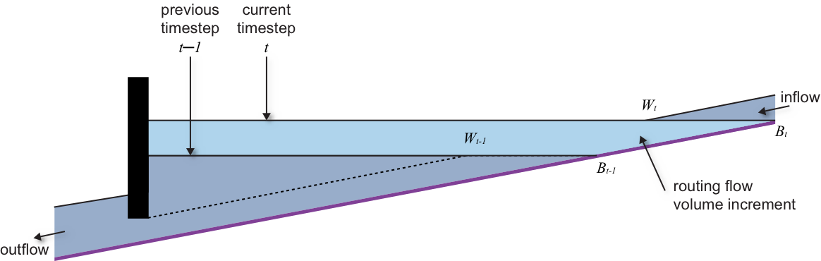
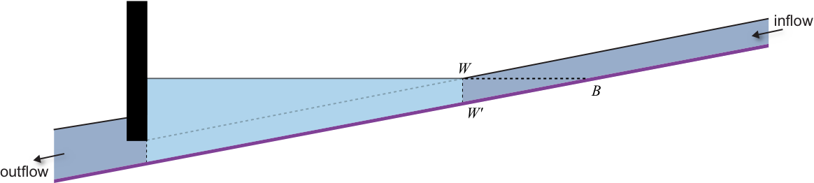
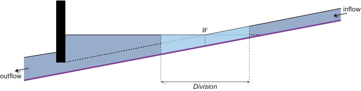
Let’s investigate the dimensions of this wedge-shaped volume and how they change as the water level rises and falls. Figure 34 represents a cross-section of the weir, with the areas and distances labelled. Because the weir storage relationship is assumed to be constant for the length of the weir, the ratios of the areas outlined in the figure are equal to the ratios of the corresponding volumes of water. The wedge-shaped volume corresponds to the lighter-shaded triangle.
Figure 34. Configuration of water in weir
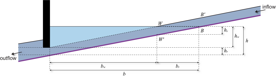
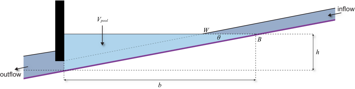
The water in the weir is regarded as made up of the water in the wedge region and the water occupying the region below the wedge, which is essentially the channel in which the water runs when the weir is not activated, and has a constant depth hr. The total depth h at the weir wall can be expressed as:
Equation 142 | 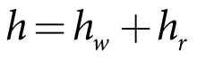 |
where
hw is the height of the wedge.
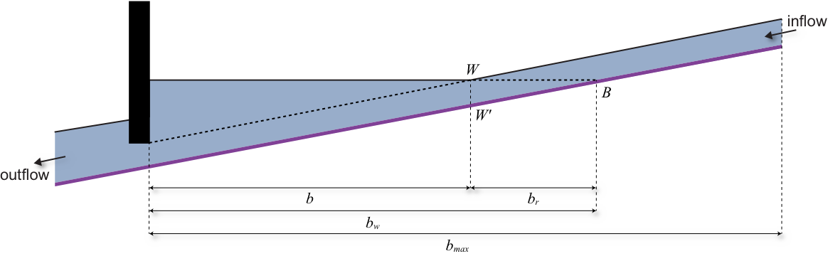
Figure 35. Weir pool
The lighter-shaded area in Figure 35 is the weir pool and its length b can also be expressed in the form:
| Equation 143 | 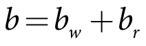 |
where
bw is the distance from the weir wall to the point W where the surface of the weir pool meets the top edge of the channel of depth hr and br is the length of the lighter-shaded triangle in Figure 36
Figure 36. Another similar triangle
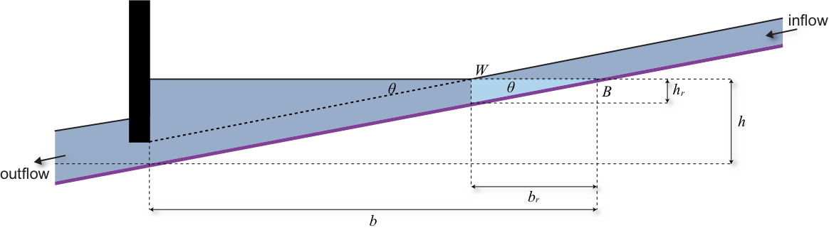
If the inflow into the weir is greater than the outflow from the weir, the surface level will rise. The points labelled W and B in Figure 34, where the surface meets the top of the routing area and where it meets the bed, respectively, will then move rightwards and upwards parallel to the river bed, causing the triangular cross-section to expand but leaving its proportions and internal angles unchanged. Also the lighter-shaded weir pool area in Figure 35 has the same interior angles, so its sides are in the same proportions too, and so are those of the small lighter-shaded triangle in Figure 36.
Hence if h and hw are the total depth of the weir pool and the depth of the wedge-shaped region at the weir, and b and bw are the length of the weir extent and the length of the top edge of the wedge, then as the wedge expands (or contracts) the ratios h/b, hw / bw and hr / br all maintain a common value D (which in fact is equal to tan θ). In particular, if hmax and bmax are the values of h and b when the weir pool reaches its maximal value, then:
| Equation 144 | 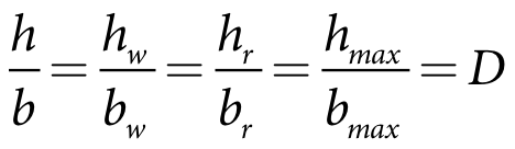 |
If Vmax is the volume of the weir pool when this maximal level in the weir is attained, then:
| Equation 145 | 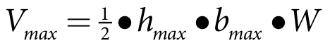 |
where
W is the width of the reach. Similarly, if is the volume of the weir pool, then
| Equation 146 | 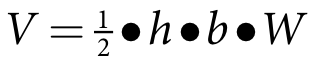 |
so that:
| Equation 147 | 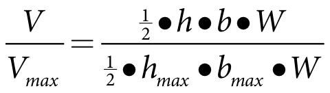 |
Using Equation 144, replace h and hmax in Equation 147 by b × D and bmax × D, respectively, and then cancel the common terms ½ and W and D. This gives:
| Equation 148 | 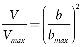 |
or, equivalently:
| Equation 149 | 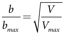 |
In words, this says that when the volume of the weir pool reaches a certain proportion of its maximal value, the length of the backflow reaches the square root of the same proportion of its maximal value.
Now Equation 144 implies that:
Equation 150 | 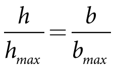 |
so Equation 149 can also be expanded to:
Equation 151 | 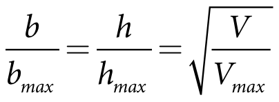 |
In exactly the same way, the volume Vw of the wedge is given by:
| Equation 152 | 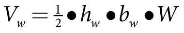 |
Divide by Equation 145 again and note that bw / bmax = hw / hmax; this yields
| Equation 153 | 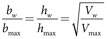 |
Finally compute in the same way the volume V0 of the wedge corresponding to the small triangle BWW’ and make the substitution hr = br × D, again using Equation 144:
| Equation 154 | 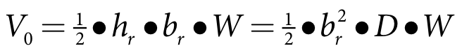 |
Dividing Equation 154 by Equation 145 gives:
Equation 155 | 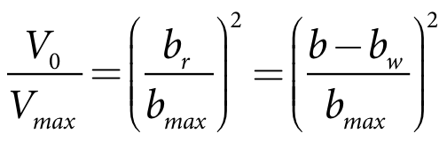 |
and this leads to an expression similar to Equation 149 and Equation 153 for the ratio br / bmax:
| Equation 156 | 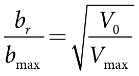 |
In applying these equations, it is convenient to choose units to make bmax = 1, so that Equation 149, Equation 153 and Equation 156 reduce to:
Equation 157 | 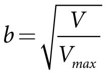 |
| Equation 158 | 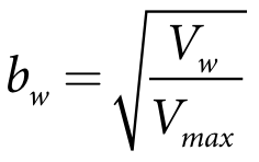 |
| Equation 159 |  |
These equations express the three distance b, bw and br in terms of corresponding volumes V, Vw and V0.
It is also useful to be able to calculate the routing depth, expressed as a proportion hr / h of the weir pool depth, in terms of the routing volume Vrouting and the weir pool volume V. This is provided by the following equation, which will be derived below:
Equation 160 |  |
With the assumption bmax = 1, Equation 160 takes the form:
Equation 161 | 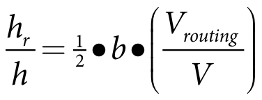 |
To establish Equation 160 , and hence Equation 162, note first that Vrouting represents the volume of routing flow when the weir pool is filled to its maximal extent - that is, when the length of the weir pool equals bmax. Since the routing depth hr is constant, the part of the routing volume situated downstream of the point B is obtained by scaling down Vrouting by the factor b / bmax (see Figure 37). That is, it is equal to:
Figure 162 | 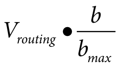 |
Next observe that, in Figure 37, the parallelogram area formed by the channel bed, a line parallel to the channel bed, the weir wall and a vertical line that intersects the channel bed at point B is twice the size of the weir pool.
Figure 37. Proportional routing height
Therefore the volume contained by this parallelogram is equal to 2 × V. The smaller lighter-shaded parallelogram representing the routing volume differs from the large parallelogram only along the vertical dimension, so the areas of these two parallelograms (and the volumes of water they represent) are in the same proportion as their respective depths - that is, in the ratio hr : h. Consequently, the value of hr / h must be the same as the corresponding fraction involving the two volumes. That is:
Equation 163 | 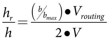 |
which simplifies immediately to Equation 160.
Finally, to obtain an equation expressing bw in terms of hr and b, recall that Equation 144 implies that hr / h = br / b, while Equation 143 implies that bw = b - br, so that:
| Figure 164 | 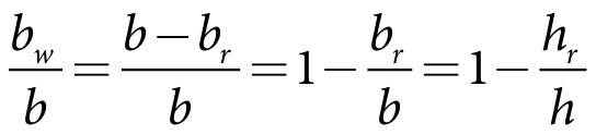 |
and hence:
| Equation 165 |  |
Modelling the flow
As usual the reach is broken down into divisions and the study of the flow involves treating the flows into and out of each division and the change in storage volume in that division, computed for each time step. This section will give a general picture of the steps involved in building the model, without going into any details.
Step 1
Routing flow
The first step again involves studying the flow in a situation where the weir gates are raised. Then the flows and storage can be computed as for a reach, where the outflow from each division is the inflow to the next. This gives us, for each division and each time step t, an inflow , an outflow and a storage volume. The outflow from the most downstream division will be the maximum outflow that can occur from the weir in the current time step.
Step 2
Calculating proportional height and back flow
Next assume that the weir gates are in place and examine the flow into the weir over a time step, assuming that at the start of the time step the water in the weir pool occupies volume and the routing volume is. To carry out further calculations we need to determine the dimensions of the weir pool at this stage.
Equation 149 shows that the proportional backflow b / bmax (to the point B) and the proportional depth h / hmax of the weir pool are given by:
| Equation 166 | 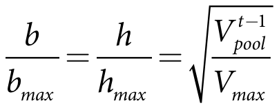 |
Now use equation Equation 164, with Vpool and Vrouting replaced by Vt-1pool and Vt-1routing, to obtain:
Equation 167 | 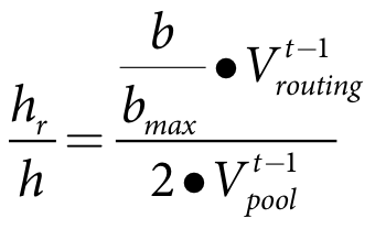 |
Next equation Equation 166 shows that the length bw of the wedge is given by:
Equation 168 |  |
Knowledge of the value of b / bmax tells us the location of the point B. The division containing B is the division in which the upstream flow enters the weir pool. If the divisions are numbered from the most upstream (number 1) to the most downstream (number ndiv, say), and B lies in the division number divinflow, then the value of divinflow is given by:
Equation 169 | 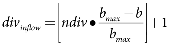 |
where
![]() denotes the integral part of x (that is, the largest integer ≤ x).
denotes the integral part of x (that is, the largest integer ≤ x).
Step 3
Calculating inflow from upstream flows (Part 1)
The inflow volume into the weir for the current time step is calculated using the routing inflow from upstream calculated in Step 1, including any calculated additional fluxes (groundwater, loss and time series), and subtracting the increment in the upstream storage between the current and previous time step, which represents the part of the inflow volume that needs to be apportioned to routing (see Figure 38). Since the upstream water enters the weir pool in division divinflow, the routing inflow from which this increment is to be subtracted is.
Figure 38. Change of weir configuration during one time step
The upstream volume for the current time step is the lighter-shaded area in Figure 39.
Figure 39. Upstream flow calculation
The volume V0 in the small region WW’B is also related to Vmax by equation Equation 159, from which it follows that:
| Equation 170 | 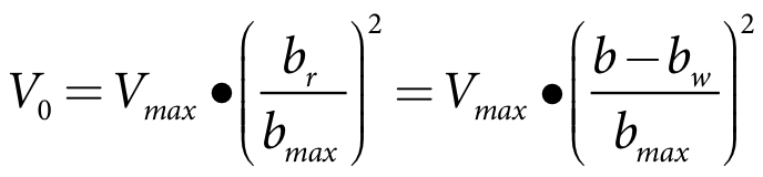 |
From Figure 39 it is clear that the volume of water upstream of the weir can be obtained by subtracting the volume V0, just calculated, from the total water volume in the routing channel beyond the vertical line through W. However, if the maximal length of the weir extent is taken to be 1, then the distance of W from the wall is bw, the horizontal extent of the part of the routing channel beyond W to the farthest point is 1 - bw. As the channel is of uniform depth, it follows that the volume filling this region is (1 - bw) × Vrouting. It now follows that the upstream volume upstreamVolcurrent for the current time step is given by:
Equation 171 | 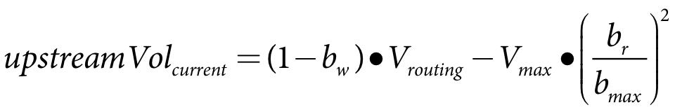 |
We also need to calculate upstreamVolprevious, the upstream volume at the end of the previous time step. Once we have this figure, then, as stated above, we can derive the inflow into the weir from the formula:
| Equation 172 |  |
However, the calculation of the upstream volume for the end of a time step (which enables us to compute upstreamVolprevious) is deferred for now, as it depends on results to be covered in the following sections.
Step 4
Updating the weir storage table
The Source storage table displays the storage volume and surface area for a number of values of the water depth.
The program adjusts the values of storage volume input by the user to account for the presence of routing volume, which is excluded from the storage calculation. The input storage volume is adjusted for every value in the table by removing the proportion of volume that needs to be reckoned as routing volume. To determine this proportion, calculations like those carried out in the previous paragraphs are performed for each row in the table. The calculation for a particular row starts with the volume figure, say V, for that row and uses it in place of the volume in equation Equation 167 to derive corresponding values for hr and b, and then calculates a value for bw from equation Equation 169. These values describe how the water is distributed in the weir pool for the particular value of V and the dimensions of the wedge and so can be used to determine the volume of the routing channel (the lighter-shaded area in Figure 40). This quantity is now subtracted from V and the resulting figure is taken as the volume for the current row.
Figure 40. Updating storage volumes
Step 5
Calculating the maximum and minimum release rates at the default outlet
The minimum and maximum operating levels are now used to adjust the minimum and maximum release curves on regulated outlets from the weir.
Assuming that the operating levels set by the user are within the regulated range of the weir, set the minimum and maximum release curves values to zero whenever their values are less than or equal to the minimum operating level on all regulated outlets. Then adjust the minimum release curve on the default outlet according the following equation, which is designed to maintain the weir operating level at the maximum operating level during periods of high flow:
| Equation 173 | 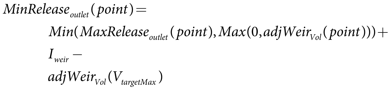 |
This means that any inflow that will cause the weir to go above its maximum operating level will be released down the default outlet path.
Step 6
Calculating the weir pool volume and the resulting release for the current time step
The calculation of the weir pool volume and the release at the end of the current time step is carried out by the same general method used for general storage nodes. It involves calculating fluxes (inflow, evaporation, groundwater, etc), as described in the storage node section. These calculations are integrated across the time step, meaning that there is no need to recalculate volumes and level for any intermediate times during the time step.
Once the volume figures have been updated, Source calculates values for the various quantities associated with the model, including net evaporation fluxes.
Step 7
Calculating the wedge dimensions based on the calculated weir pool volume and routing volume at the end of the time step
At this stage we know the weir pool volume and we know that any changes to the volume must produce a corresponding change in the size of the wedge, but we need to determine the actual dimensions of the wedge at the end of the step. For this we simply repeat the calculations of Step 2, but substitute the volume Vtpool in place of Vt-1pool. Equation 167 now becomes:
Equation 174 | 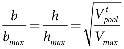 |
Next use Equation 164, replacing V and Vrouting by Vtpool and Vtrouting, to derive an expression for hr / h:
Equation 175 | 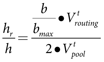 |
which can be used to give an expression for bw:
Equation 176 | 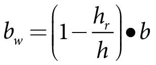 |
Step 8
Determining the impact of the changes to the wedge on each division and adjust the net evaporation calculations as necessary
After carrying out Step 4, we can determine Otweir, the total weir outflow volume from all outlets, at the end of the time step. To determine the wedge volume Vtwedge we subtract Otweir from the overall estimated routing volume Otrouting from Step 1:
| Equation 177 | 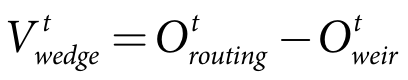 |
The calculation of Otrouting described in Step 1 includes providing an estimate of the net evaporation flux Evtrouting (div) for each division. In addition it was mentioned in Step 6 that a net evaporation flux Evtstorage is also calculated for the weir pool after the storage table is updated. However, these two kinds of estimate are calculated independently and need to be combined into a single figure for each division, reflecting the relative proportions of weir storage volume and pure routing volume that make up the total for that division. This is done is by a procedure that loops through the divisions, starting from the most downstream one and working up to the most upstream one, and derives a suitable evaporation figure for each division in turn. The following paragraphs outline the procedure, suppressing some details.
For each division the relative contributions of Evtrouting (div) and Evtstorage are initially assigned as follows, depending on where the point W (where the wedge meets the routing channel) is situated in relation to the division. There are three cases:
- W is upstream of the current division. In this case, the division lies entirely within the weir pool and the net evaporation flux is taken to be a fraction of Evtstorage, calculated according to the relative extent of the weir pool occupied by the division - that is, Evtstorage × (length of division)/(length of weir pool).
- W is downstream of the current division. In this case, the division is entirely upstream of the weir pool and the net evaporation flux is taken to be just Evtrouting(div).
- W lies inside the current division. This is the case shown in Figure 42. In this case the division overlaps the edge of the wedge and the net evaporation flux is taken to be a weighted combination of Evtstorage and Evtrouting(div), the weights being assigned to reflect the relative volumes associated with each of the two shaded areas - that is, according to the relative distances of W from the downstream end of the division and from the upstream end of the division, respectively.
The rules just described assign an initial value to the net evaporation flux. However, before processing the next division certain adjustments are made to the wedge volume Vtwedge to ensure that the net evaporation flux just calculated does not deviate too much from the initial routing estimate. These are then carried forward into the next step of the processing and the corresponding total volume Vt(div) in the division is stored.
Figure 42. Allocating evaporation components according to volumes
At the end of the iterative procedure, the figure upstreamVolprevious can be calculated. First add the stored values Vt(div) from each division:
| Equation 178 | 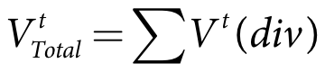 |
where
ndiv is the number of divisions.
Then, using the weir pool volume Vpool calculated in Step 6, we set:
| Equation 179 |  |
Step 9
Calculating inflow from upstream flows (Part 2)
Now that the values of upstreamVolcurrent and upstreamVolprevious have been calculated, in Step 3 and Step 8 respectively, we can now substitute these values in equation Equation 173 and derive an expression for the inflow Itweir into the weir in the current time step.