Note: This is documentation for version 4.11 of Source. For a different version of Source, select the relevant space by using the Spaces menu in the toolbar above
Storage Node - SRG
You can change between the Backward Euler reservoir routing methods (default) and the Piecewise-linear Integral in Scenario Options » Storages.
Storages are used to hold water for varying periods. They include dams and other reservoirs; weir pools; urban detention, retention or retarding basins; and natural lakes. In regulated river systems, storages control the supply of water to consumptive and non-consumptive users, and may also provide flood mitigation and environmental services. Typically, inflows to storages include stream flow from upstream catchments, rainfall over the storage surface area, recharge from groundwater, and runoff from the local catchment surrounding the storage. Outflows from storages include controlled releases and spills. Losses from storages include evaporation from the storage surface area and seepage to groundwater.
Controlled releases from a storage include discharge via regulated outlet structures such as gated spillways, valves, pumps and gates. The amount of water released is dependent upon downstream demands, storage operating rules and maximum and minimum release constraints. In river systems with ownership, releases are also influenced by owners’ shares within the storage and the ownership of the outlet capacity.
Spills via gated spillways are modelled by specifying a minimum release for the gated spillway as a function of reservoir level. Pre-releases for flood control may be modelled using either the minimum release functionality of the gated spillway or a minimum flow node, for more complex pre-release rules such as seasonal targets.
Uncontrolled spills occur when a storage fills above the minimum level of an un-gated spillway, or the capacity of the gates on a gated spillway to control outflows is exceeded. Uncontrolled outflow may also occur through an uncontrolled outlet such as an ungated pipe culvert and via leakage through the dam wall.
The modelling of the physical operation of storages in Source is described below. Other functionalities related to storages are described in other SRG sections; these functionalities include:
- Resource assessment and water allocation
- Ownership
- of storage volume, inputs, losses, spills and outlet capacities
- Internal spilling between owners
- Internal ceding (transfer from one owner to another based on agreed protocols)
- Local borrow and payback systems.
- Weir operation (where the routing of flows in the headwater is significant - ie long flat weir pools)
- Ordering
- Storages in series (orders passed upstream and transfer between storages),
- Storages in parallel (choice of supply storage, optimisation of order delivery).
- Water quality in storages.
The ability to model the physical behaviour of storages is essential for fulfilling one of the primary purposes of Source, which is to model regulated river systems.
Scale
This node, in common with all others, is treated as a point location even though the storage represented may have large dimensions. It can therefore be considered to be site scale. It is used at every model time-step.
Principal developer
eWater Solutions, Department of Primary Industries, New South Wales
Scientific provenance
The level pool approximation for simulating the attenuation and delay caused by a reservoir has been used from the earliest days of engineering hydrology (beginning of the 20th Century).
Version
Source version 4.1.1
Structure and processes
Assumptions:
- The solution technique used assumes inflows, loss and gain fluxes, and outflows are averaged over a model time-step. This is consistent with the approach used in other parts of Source, such as link routing;
- The storage reservoir is assumed to have a level pool; and
- Relationships between storage water level, volume, surface area, and outflows are defined in terms of piecewise linear, monotonically increasing coordinate sets.
Theory
Approach
Source uses an implicit (backward) Eulerian approach for link storage routing. It assumes that the flux averages over a time step are a function of the state at the end of the time step:
Equation 1 |
|
We also use the same approach for reservoir routing. Source assumes that all reservoir variables are a piecewise linear function of the reservoir's volume. For a time step the usual applies:
Equation 2 |
|

Where Out consists of a number of components:
- Nett Evaporation
- Seepage
- Release
- Spill
And where ε is the mass-balance error.
Release and spill are the sum of the water flowing downstream in all of the outflow paths. For each path we have two relationships:
Equation 3 |
|
Equation 4 |
|
So the flow down each path will be:
Equation 5 |
|

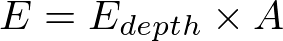
The nett evaporation is:
Equation 6 |
|
Equation 7 |
|
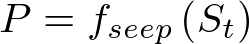
Seepage:
Equation 8 |
|
Combined this gives us the mass balance equation:
Equation 9 |
|

Parameterisation
The geometry of the storage is specified by user provided piecewise linear relationship between
- height and storage,
- height and surface area
- height and seepage.
For each outlet
- height and minimum rate of release, and
- height and maximum rate of release.
Outlets on the same path are combined into effectively one outlet.
From the user provided relationships, a common set of heights is used to calculate volume relationships for each component.
Manual Override of Releases, Levels and Ownership
Gauged releases are handled by replacing the orders in the model with the user specified time series, with the same constraints. If there is an ownership system in place, you can choose to set the ownership of the releases. If you choose to override ownership, orders are changed to match the user specified ownership.
Gauged levels are handled by using the user specified time series to adjust the storage volume. When there are multiple owners, differences between the simulated and user specified storage volumes are shared to owners according to evaporation and rainfall sharing rules.
Implementation
The following explains how the mass balance equation (Equation 9). As all of the functions are piecewise-linear we can construct a table with entries for each unique value of volume that appears in the functions:
Equation 10 |
|
The corresponding values of the min/max release, seepage and area are then calculated by interpolating the user specified values.
Table 1. Example of pre-computed solution table
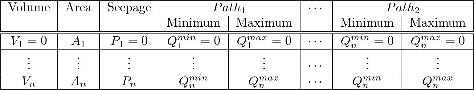
These values stay the same for the length of the model run and can then be used at each time step. Using the current value of Ordersj and Edepth we can calculate the corresponding value of ε for each table row (V):
Equation 11 |
|
At which point storage routing becomes a table lookup and interpolation exercise where we find the value of V that give a ϵ value of zero. Obviously we don't have to calculate the entire table but just use a standard search technique.
Exceptions
There are a number of special cases where the above method will not work.
Figure 1 Maximum and minimum release curves for a single outlet path
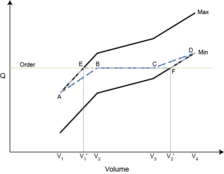
Figure 1 shows the minimum and maximum possible releases for a single outlet path with the current order for this path. Using the table search approach described above the resulting curve will be ABCD as these are the points calculated in the table. However the true curve is AEFD meaning that solutions in the range V1 to V2 and V3 to V4 will be incorrect. To avoid this we would check to see if any of the outlet's minimum or maximum curves were intercepted by their orders and if they did we would continue the table search by creating virtual entries (V1', V2', …).
While searching the table we can end up with two situations:
- We get to V = 0 and ε > 0
- We get to Vn and ε < 0
The first situation can happen when the storage has a flat bottom (ie: the storage can dry out due to evaporation but there is not enough water to meet all of the evaporative requirements). In this case the solution is a storage volume of zero and the reported evaporation has to scaled back to match.
The second situation is due to the user supplied relationship not covering a large enough range of volumes. Provided that the orders are not out-ranging the table then a solution can be obtained by extrapolating the last segment of each of the relationships.
Multiple outlet priorities
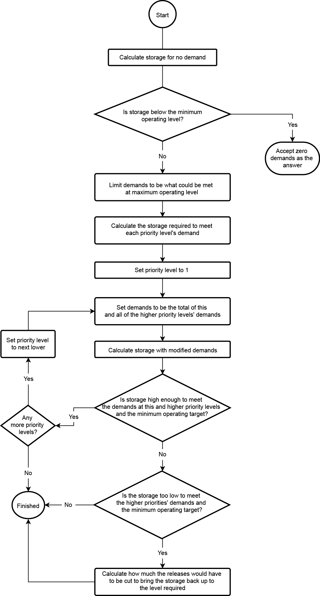
The user can assign priorities to outlet paths, which will result in shortfalls being assigned to lower priority paths. Otherwise, shortfalls are either shared evenly, or on the basis of priority ordering. An overview of the process for calculating multiple outlet priorities is shown in Figure 2, with details of the processes for reducing releases and increasing releases shown in Figure 3 and Figure 4. The methodology works by solving the timestep in the same way as if there were no priority and then checking to see if the resulting answer is outside the allowable range or if there are any outlet restrictions (Figure 2). If there are restrictions or the resulting storage volume is below the minimum allowed then an iterative approach is used when priority levels are added and trialled until there is a supply failure at which point the fraction of the last priority level that can be met is calculated (Figure 3). If the resulting storage is higher than the maximum allowed then the releases are increased in the same manner as for the case of no priorities (Figure 4).
Figure 2. Multiple outlet priorities, Process overview
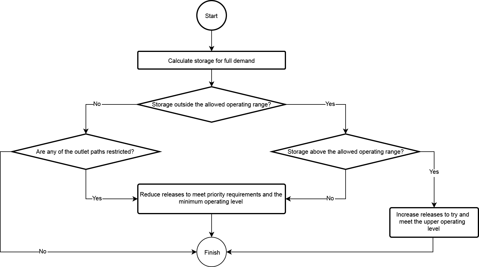
Figure 3. Multiple outlet priorities, Process for reducing releases to meet priority requirements and the minimum operating level
| Figure 4. Multiple outlet priorities, Process for increasing releases to try and meet the upper operating level
|
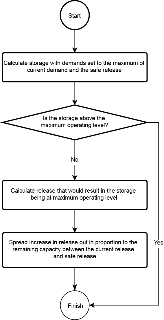
Operating targets
Solving the current time step using the above method.If the reservoir has either or both a minimum and maximum operating target we can deal with this by:
- Check to see if the resulting reservoir volume is outside the range allowed (otherwise the solution from step 1 is acceptable and we can stop).
- If it is outside of the range allowed then see if it is possible to get back into the acceptable range by either:
- If initial solution is below the minimum target then recompute the time step assuming that there are no downstream orders
- If initial solution is above the maximum target then recompute the time step assuming that the downstream orders are the greater of the current order and the maximum flow rate allowed on each outlet path for releasing above target water (the safe release).
- If the resulting answer from step 3 is still outside the allowed range the result obtained at step 3 becomes the final answer for this time step.
Compute a total release from:

Where Starget is the appropriate minimum or maximum target volume (are you trying to cut back releases to stop the reservoir dropping below the minimum or increasing releases to stop it going over the maximum).- To calculate the corresponding release rates for the solution obtained at step 5 we have to scale up or down the orders so when we evaluate equation (5) we'll get the required results. The two cases are:
- If the initial solution (step 1) fell below the minimum target volume then we are cutting back and Starget at step 5 was Smin. We cut back each path in proportion to how far their order is above fjminSmin.
Calculate the sum of current demands in excess of the path minimum capacity (limiting to the maximum outlet capacity at the minimum target volume):
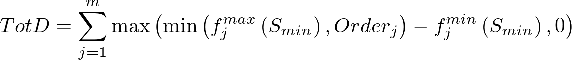
Calculate the release cutback required:
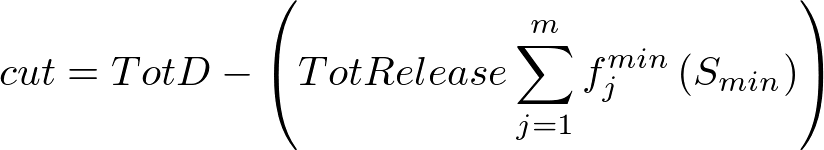
Scale back the orders:

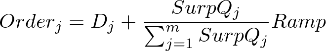
- If the initial solution (step 1) fell above the maximum target volume then we are ramping up the releases and Starget at step 5 was Smax. We add onto each path in proportion to how much remaining release capacity each path has.
Calculate maximum we can currently send down each path:

Where AllowedQj is the maximum permitted release down path j for above target water.the flow that's already going to go down path j:

the remaining release capacity:

The required increase in release is then:
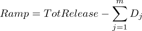
Modified orders are then calculated from:
- If the initial solution (step 1) fell below the minimum target volume then we are cutting back and Starget at step 5 was Smin. We cut back each path in proportion to how far their order is above fjminSmin.