Note: This is documentation for version 5.0 of Source. For a different version of Source, select the relevant space by using the Spaces menu in the toolbar above
Calibration Wizard for catchments
Introduction
The Calibration Wizard is used to calibrate the streamflow characteristics of a Source model. It can be used to calibrate rainfall runoff, constituent and link routing models and is primarily intended for use in unregulated systems. Much of the functionality relies on characteristics of catchments scenarios - specifically the presence of a sub-catchment map.
In summary, the steps involved in undertaking calibration analysis are:
- Launch Source, open your project, and then open the scenario you wish to calibrate;
- Start the wizard and work through its steps (see Calibration Wizard below);
- Click Run on the Simulation toolbar to perform a calibration run; and
- Examine the results.
Characteristics
The calibration wizard offers a lot of flexibility. It supports:
- Calibrating to single or multiple observation gauges;
- Multiple gauges in different parts of the catchment (parallel) or nested (i.e. upstream/downstream);
- Ability to calibrate modelled flow at points or links (downstream flow), and the point can be node or outlet of catchment;
- Ability to calibrate modelled constituents at points or links, and the point can be node or (outlet of ) catchment;
- Equal weighting between gauges or different weightings (e.g. by area, length of observed record, or quality of observed record);
- Automatic calibration using a mathematical optimiser and an objective function, or manual calibration using objectives functions and visual inspection;
- Compound objective functions including the ability to manipulate weighting between objective components;
- Ability to calibrate multiple gauges for the same time period or different time periods;
- Ability to group parameters across the catchment or keep them independent, with the ability to choose this for each parameter; and
- Ability to calibrate rainfall runoff models or link flow routing models or to calibrate them at the same time.
- Ability to calibrate constituent model.
The Calibration Wizard is organised as a step-by-step process, which guides you through configuring the model for calibration, and a Calibration Runner, which handles the actual calibration, either in an automated fashion using an optimiser, or manually, with the ability to directly specify parameter values.
Calibration Wizard
To start the wizard, choose Flow Calibration Analysis from the Select Analysis Type popup menu on the Simulation toolbar and then click Configure, which is also on the Simulation toolbar. The wizard comprises of four steps:
- Calibration targets -define model elements ( e.g. catchment, node or link) and associate them with the observed data loaded in the model , and select the objective function(s) that you want the optimiser to use to assess how well it fits (Figure 1);
- Period definition - define the time period(s) for your calibration. When you have more than one observation data set, you can define a distinct calibration period for each gauge. You also define a warm up period, where the overall model simulation starts at some point in time before the first calibration period commences (Figure 2);
- Metaparameter definition - define parameters that will be modified during the calibration to improve the model fit to the observed data. Metaparameters are distinct from the actual parameters in the model. They can correspond directly to model parameters, or multiple model parameters can be grouped together to match a single metaparameter. Usually some combination of these approaches is used to reduce the number of parameters being calibrated, while retaining distinct parameters where it is expected to improve the fit (Figure 3); and
- Select optimisation function - choose and configure the optimisation strategy, including the option of using manual calibration in lieu of optimisation (Figure 4).
Configure Calibration Points ( previous Select elements to record )
In the first wizard step, you define the point(s) or link(s) in the model where you will be calibrating to observed data (Figure 1). You can select (the outlet of) catchments, nodes or the downstream end of links, or miscellaneous if applicable. For each of these points you associate observed data and optionally provide a site weighting. You also define your calibration objectives at this step, including optionally weighting different components. You can set up the wizard to calibrate downstream from the link ,or at a node, or at the outlet from a catchment. Similarly, you can calibrate the modeled constituents.
You can select either a node or link on which to load observed data using either the Project Hierarchy or clicking the element in the geographic editor panel. The steps to load time series at a Gauge for which you have observed data are similar for a link:
- Click the gauge node in the geographic editor panel so that it becomes selected;
- Click observed flow and select Data Source radio button;
- Choose the time-series of its associated observed data from Data Sources frame; and
- Click OK.
The same method is used to load time series for links as well.
Figure 1. Calibration Wizard (Configure Calibration Points)
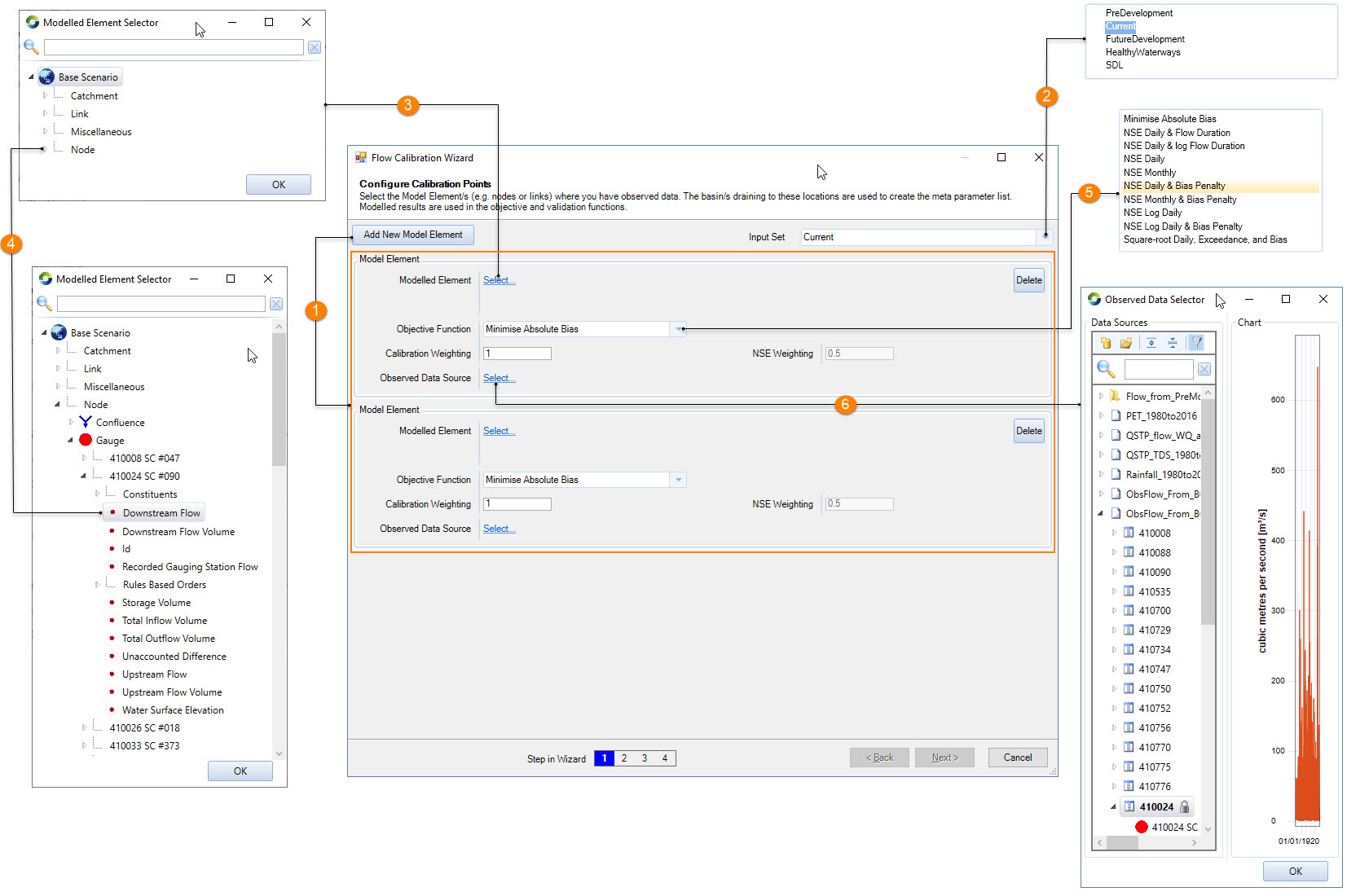
At the beginning, the interface of Step 1 in Flow Calibration Wizard (i.e. the central Windows of Figure 1) only has two components (i.e. Add New Model Element button and Input set drop down list):
Add New Model Element button is used to add a modelled element (node or link or catchment) where the observed data was loaded in Data Sources of the Source model and calibration can be performed. Clicking on this button (action 1) will add one frame of Model Element to the interface.
The user can have multiple frames of Model Element. In another word, the user can select multiple model elements (e.g. nodes or links) for the calibration at same time.
Input set drop down list allows the user to select an available Input Set for the calibration (action 2).
In each added Model Element Frame:
Model Element | Select… can open Modelled Element Selector windows by clicking on Select… (action 3). The user can navigate Modelled Element Selector windows to select the required calibration element and parameter by clicking on the triangle symbol (action 4). For example, the action 4 in Figure 1 is to select the modelled downstream flow at gauge 410024 to calibrate.
Delete button in each frame of Model Element can remove that frame from the interface. It will also remove the element, which is defined by that frame, from the calibration.
Objective Function drop down list can be used to define the calibration objective(s) (action 5 ). Your choices are:
- Minimise Absolute Bias
- Bivariate Statistics SRG#FlowDuration
- Bivariate Statistics SRG#LogFlowDuration
- NSE Daily
- NSE Monthly
- Bivariate Statistics SRG#BiasPenalty
- Bivariate Statistics SRG#BiasPenalty
- NSE Log Daily
- Bivariate Statistics SRG#BiasPenalty
- Bivariate Statistics SRG#SDEB (previously called Sum of Daily Flows, Daily Exceedance (Flow Duration) Curve and Bias) (SDEB)
In most cases, model calibration seeks to maximize the selected objective function. The exceptions are the Absolute Bias and SDEB, which are minimized.
The general Objectives in Source are described in (Calibration analysis - SRG). The term and algorithm used in those objective function such as NSE, bias can refer to following links:
- Bivariate Statistics SRG#SutcliffeEfficiency
- Bivariate Statistics SRG#NSEofLogData
- Relative Bias
- Bias Penalty
- Bivariate Statistics SRG#PearsonsCorrelation
- Bivariate Statistics SRG#NSEofFlowDuration
- Bivariate Statistics SRG#NSEofFlowDurationofLogData
Observed Data Source | Select… can open Observed Data Selector interface by clicking on Select… (action 6). The Observed Data Selector interface allows the user to select the observed data corresponding to the selected element and parameter. The observed data need to be loaded in the Data Sources already.
Calibration Weighting box allows you to define an alternative weighting between the objective functions defined for the elements, where you have multiple elements such as gauges. The default is 1 for each gauge, so each gauge would contribute equally to the overall objective function. The use of Calibration Weighting is optional, and the meaning of the weights can be defined by you. You might use this in a situation where for instance, there are 20 years of data at one gauge and 10 years of data at another, then apply a weighting of 2 to the first gauge and 1 to the second gauge. Alternatively, you might place higher weighting on observation points that represent more of the catchment area.
NSE Weighting box can be used to change the weighting between the components of composite objective functions. The value should be between 0 and 1 and is applied to the "first" component of the compound objective - i.e. in NSE with log flow duration, the weighting you specify will apply to a "regular" Nash Sutcliffe efficiency on the observed and predicted data (1-Weighting) and will apply to the NSE on the logged flow duration curves.
When you have finished loading time series, click Next.
Define calibration period
In this wizard step, (Figure 2), you define the period over which the calibration should be performed for each observation site.
Figure 2. Calibration Wizard (define calibration period)
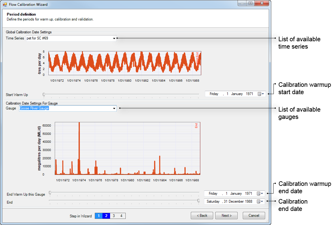
The following dates are required:
The start and end dates for the overall simulation, which is constrained by the available input data (typically climate records) - with the goal of providing a warm up period for each gauge. The Simulation End Date is automatically set to the latest Calibration End Date; and
The Start and End dates for calibration at each site, which are constrained by the available observation data for the site - allows the calibration to take place over a subset of the observed data. This might be in order to save some data for validation, or to filter out poor quality observations.
Source provides Start date and End date values which represent the lowest common denominator of the time series you loaded in the preceding step and all other input time series that have been used within the Source model (such as rainfall and evaporation data). Source also proposes a warm-up period; calculation of the objective function for the calibration commences after the simulation reaches the Warmup end date. You can adjust all dates as required and then click Next.
As an example, consider the calibration of a model with a climate record from 1 January 1950 to 31 December 1999 (as shown in Figure 3). There are two observations sites, with the following observed streamflow records:
- S1: 1 January 1960 - 31 December 1989; and
- S2: 1 January 1975 - 31 December 2010.
Figure 3. Timeline for calibration period
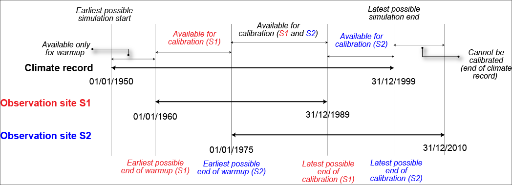
Consider the following valid calibration periods:
- S1 starts on 1/1/1960 and ends on 31/12/1989; S2 starts on 1/1/1975 and ends on 31/12/1999 - for a simulation start date of 1/1/1959 and end date of 31/12/1999, the calibration periods of both S1 and S2 are valid as they fall within the simulation period; and
- S1 and S2 have the same start (1/1/1975) and end (31/12/1989) dates; the simulation start and end dates are 1/7/1974 and 31/12/1989 respectively - a subset of both S1 and S2 are used with a 6-month warm-up period for both records.
 The period from the start date to the warm up end date should be sufficiently long to ensure that the soil moisture and groundwater stores represented within the rainfall runoff models have a sufficiently long warm up run period. That way, the volume of water in each of the stores will not be influenced by the volume that was set within those stores at the start of the warm up period. For most catchments and models, a warm up period of between 3 and 12 months should be sufficiently long for this to occur. |
Working with metaparameters
In the calibration tool, metaparameters are parameters defined specifically for the purposes of calibration, with each metaparameter mapping to one or more parameters in the underlying model. In this way, metaparameters allow you to selectively reduce the number of independent model parameters that need to be calibrated. Each metaparameter defines the allowable ranges across which each of the associated model parameters can be varied as the calibration executes. Any model parameter which is not associated with a metaparameter will not be varied during a calibration run and will remain at the same value as it was set to during the set up of the model via the Edit menu before entry into the wizard.
Metaparameters can be extremely fine-grained with a one-to-one relationship between a metaparameter and a model parameter, coarse-grained where a single metaparameter controls all the like-named model parameters in the model, or anything in between. Metaparameters are created by grouping one or more like-named model parameters and, accordingly, it can be helpful to treat metaparameter and group as synonyms.
In Source, each node, link, catchment and functional unit is a model in its own right, with its own, independent parameters. Thus, even when a catchment model is built using a rainfall runoff model with a small set of parameters, such as GR4J which has four parameters, the application of the model across multiple functional units in many catchments has a multiplicative effect on the number of model parameters. |
Defining metaparameters
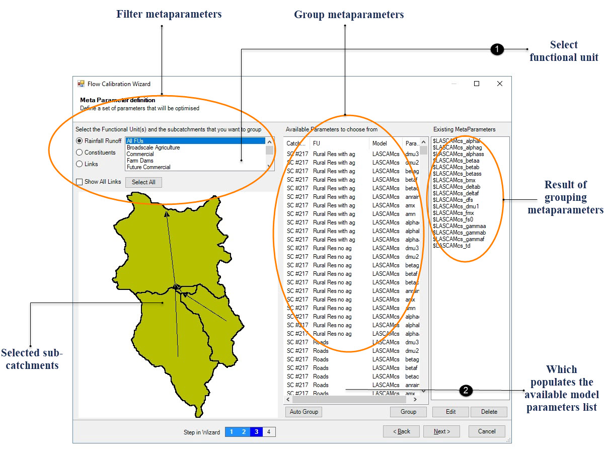
The Metaparameter definition dialog (Figure 4) is divided into three columns, representing three main steps:
- Filter - allows you to specify a subset of the model, for consideration when configuring metaparameters. Depending on the type of metaparameters you wish to define, enable the Links (for links), or Catchments (for rainfall runoff models) , or Constituents ( for Constituent models) radio button. Then, click (or use Shift+Click to select multiple areas) on the coloured area of the sub-catchment to highlight it.;
- Group - choose how to group metaparameters, either mapping to individual ones, or grouping multiple metaparameters. These appear in the third column (Result); and
- Result - here, you can make alterations to metaparameters (such as changing the calibration range for each metaparameter) selected under Group.
This process of defining metaparameters is iterative, and can be used for a variety of application, ranging from links and rainfall runoff models to different FUs or for different locations in the model.
Figure 4. Calibration Wizard (view available parameters)
In the calibration tool, metaparameters are parameters that are defined specification for the purposes of calibration, with each metaparameter mapping to one or more parameters in the underlying model. In this way, metaparameters allow you to selectively reduce the number of independent model parameters that need to be calibrated. Each metaparameter defines the allowable range across which each of the associated model parameters can be varied as the calibration executes. Any model parameter which is not associated with a metaparameter will not be varied during a calibration run and will remain at the same value as it was set to during the set up of the model or via the Edit menu before entry into the wizard.
Creating metaparameters
In addition to the process outlined in Defining metaparameters, you can also create metaparameters using the Auto Group button. Auto-grouping creates one metaparameter for each distinct type of model parameter. After clicking Auto Group, the list of available model parameters will always be empty – for that combination of functional units and sub-catchments.
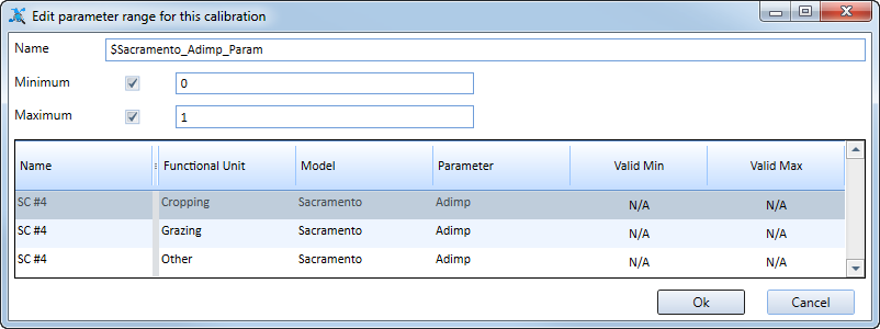
The name of each metaparameter is constructed from the name of the model parameters with which it is associated. This may produce naming collisions where the same model parameter name is used in different types of functional unit. To avoid a naming collision, you may need to rename one or more metaparameters to make them unique. To rename a metaparameter and/or edit parameter ranges, first select the metaparameter and either double-click the metaparameter or click Edit to open the dialog shown in Figure 5. Then:
- Edit the Name field so that the name is unique. To differentiate between parameters that have the same name, but are from different FUs, enter a suffix at the end of the parameter;
- Specify the Minimum and Maximum fields - the are defined target ranges for a calibration. Default values are included when you open the dialog; and
- Click OK.
Figure 5. Calibration Wizard (Edit metaparameter)
You continue the process of creating metaparameters until all of the model parameters you wish to have varied during the calibration run have been associated with metaparameters, or the list of available model parameters is empty. Remember that the available parameters list depends on your FU and sub-catchment selections.
Creating metaparameters for rainfall runoff models or Constituent models
To create a metaparameter for a rainfall runoff model/Constituent model:
- Select one or more functional units (Figure 4). You can add functional units to the selection using either the shift or control keys. You can select all functional units by clicking All FUs.
- Select one or more sub-catchments. (a) If you select a node in Figure 1 , only associated upstream catchments are displayed on the map in Figure 4 and you can easily to define to catchment(s) using Select All button. (b) if you define a point from Catchment in Figure 1, you can add sub-catchments to the selection using the Control key or by dragging an extent across the map of catchments. Whenever at least one FU and one sub-catchment is selected, a list of available model parameters will be displayed in the middle panel. A model parameter is only available in the middle panel if it is not already associated with a metaparameter. This process can be repeated for links.
- From the list of available model parameters, select one or more like-named parameters. You can add model parameters to the selection using either the Shift or Control keys.
- Click Group. This creates a metaparameter and associates it with the selected model parameters. The selected model parameters are then removed from the list of available model parameters.
To calibrate parameters of link routing models, ensure that storage routing has been configured for the desired link. When defining metaparameters, click on Links (left-hand side of Figure 4) to list the link related metaparameters and carry out the same process outlined for rainfall runoff models. Ticking Show All Links box will display all links on the map in Figure 4.
Once you have finished defining and editing metaparameters, click Next.
Adjusting metaparameter ranges
You can adjust the range over which the associated model parameters are varied using the EditMetaParameter dialog (Figure 5). To adjust a range:
- Select the metaparameter to be edited in the list of metaparameters;
- Either double-click the metaparameter or click Edit;
- Adjust either or both of the Min and Max fields; then
- Click OK.
Configure optimisation functions
In this wizard step you choose an optimisation function (Figure 6) and then adjust its parameters. The available optimisation functions are:
- Shuffled Complex Evolution (SCE) - a global optimiser that learns the parameter set for calibration from previous runs;
- Uniform Random Sampling - another global optimiser that randomly selects a parameter set from the available metaparameter list and runs the model. It then picks the best as the calibrated set. One disadvantage is that it does not learn as the process progresses;
- Rosenbrock - a local optimiser; and
- Manual optimisation - allows you to manually edit metaparameter values.
Figure 6. Calibration Wizard (Configure optimisation function)
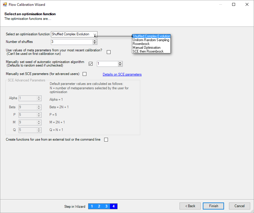
If you enable the Use values of meta parameters from your most recent calibration? checkbox, this will use the current metaparmaters as the starting point for the optimisation algorithm during the next round of calibration.
A typical example would be at the completion of metaparameter optimisation using SCE, the "best set" of metaparameters is used as the initial parameter set or "seed" for fine-tuning the metaparameter range using the Rosenbrock optimiser. All optimisation functions allow you to set a limit on the number of iterations. Shuffled Complex Evolution offers additional parameters but these should be left at their default values.
If you enable the Manually set seed of automatic optimisation algorithm checkbox, this will use the entered value (1 in Figure 6) as the seed for the calibration, otherwise a random seed is used. This is useful for testing and debugging.
Shuffled Complex Evolution
The Shuffled Complex Evolution-University of Arizona (SCE-UA, or often just SCE) is an efficient global optimiser that is commonly used for many models, including rainfall runoff models.
The SCE algorithm is designed to optimise the metaparameters that are assigned for the models within Source. It has its own parameters that control the optimisation process. The algorithm involves selecting a number of sets of metaparameter values at random. The model is run and the objective function is calculated for each of these sets of metaparameter values. The sets of metaparameter values are formed into a number of groups, or "complexes". The user can control:
- P - the number of complexes to be run; and
- M - the number of sets of metaparameters in each complex.
During the first step of optimisation, the optimiser will select, at random, P multiplied by M metaparameter sets and evaluate the objective function for each of those metaparameter sets.
Following this, the complexes are shuffled with metaparameter sets randomly redistributed into new complexes. At this point, there is a process of competitive complex evolution. In this step, new metaparameter sets are derived from the metaparameter sets within each complex. The evolution is competitive because although there is a random selection, the metaparameter sets that return better values of the objective function receive higher weighting in the selection process and are therefore more likely to be selected. The new evolved metaparameter sets can (at random) replace the metaparameter sets that were within each of the original complexes.
The number of shuffles (i.e. the number of times that the SCE process is completed) is set by the user.
There are three parameters that control the complex competitive evolution process:
- Q – the number of metaparameter sets that are selected at random from within each complex to form the parents for the evolution process;
- α – the number of times that mutation of parameter sets should be attempted; and
- β – the number of new offspring that should be generated within each complex.
The parameters have default values as defined below, but you can change these values when you enable the Edit advanced SCE parameters (for advanced users) checkbox:
- α = 1;
- β = 2N + 1;
- P = 5
- M = 2N + 1;
- Q = N + 1
where N = number of metaparameters selected by the user for optimisation.
There is no specific guidance on P, the number of complexes, other than that it should be greater than 1. In practice, a value between 4 and 8 would be appropriate, and Source uses a default value of 5. For example, if you have 10 metaparameters in your model and you select M = 21 (in accordance with the above guidance) metaparameter sets in each complex, and select 5 complexes (P = 5); then the first 105 iterations of the model are all randomly sampled from within the feasible parameter space. Only at this point, would shuffling occur and new parameter sets be generated via the competitive complex evolution process.
The number of shuffles, along with the other parameters, controls the maximum number of iterations that the model will be run for.
Manual optimisation
Manual optimisation allows you to manually edit metaparameter values, and then run the model. Choose to open the Simulation Runner dialog. Click on the Create new meta parameter set button and enter the desired metaparameter values in the appropriate column in the Meta parameter set editor table. Click on Simulate with current meta parameter set to start the calibration.
Calibration Runner
Click Finish to complete the wizard. If you need to make changes in any of the preceding steps, start the wizard again as described under Calibration Wizard, click Next until you reach the appropriate screen, edit as needed, then click Next until you reach the end of the wizard, and click Finish. An alternative method is to select a specific step of the calibration wizard from .
Once a scenario has been configured for a calibration run using the wizard, you can start the calibration simulation run. Click Run on the Simulation toolbar. The Simulation Runner dialog (left of Figure 7) opens and the calibration run begins.
Figure 7. Calibration Wizard (simulation runner)
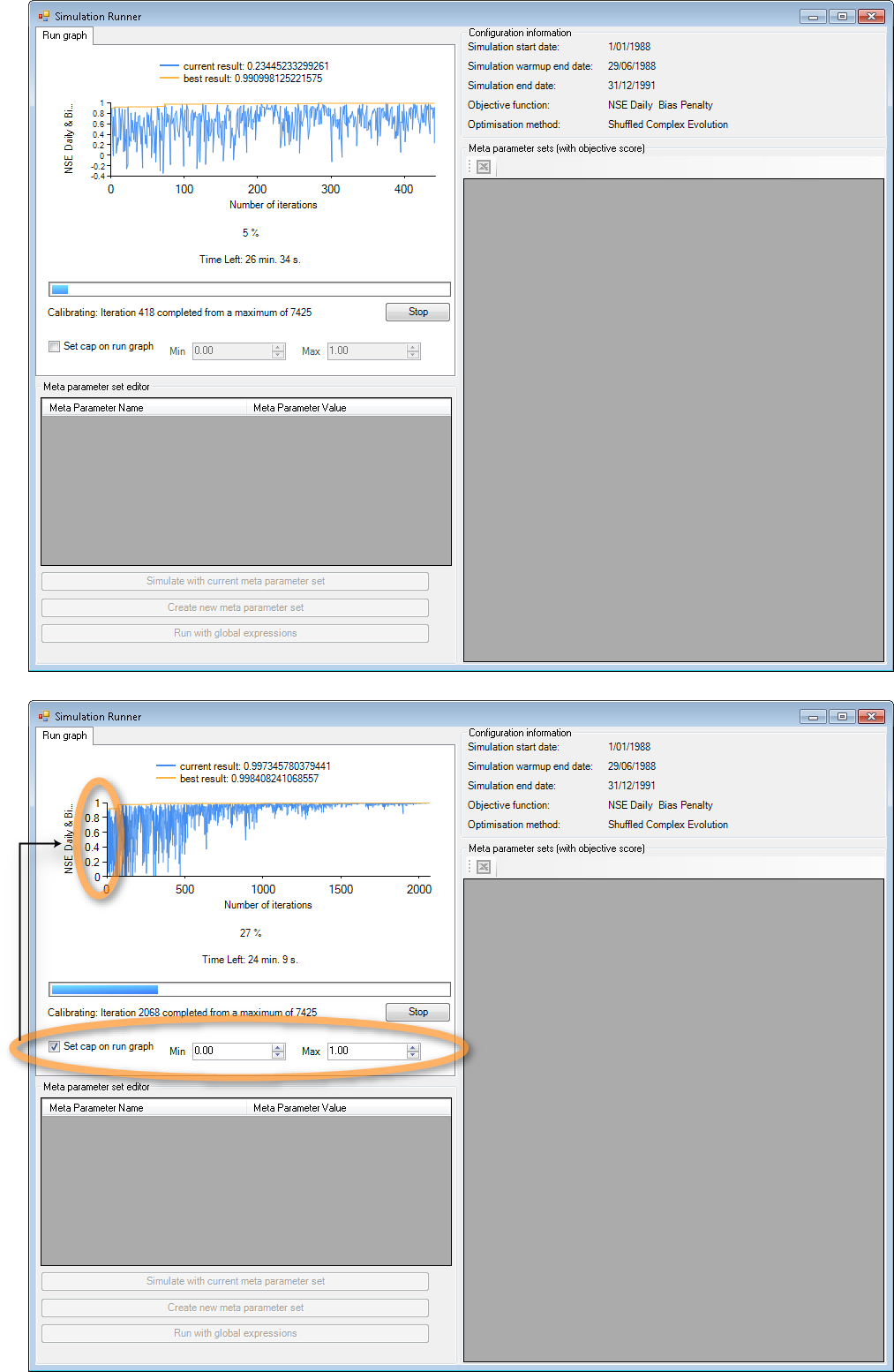
A calibration run is a series of iterations. By default, the iterations will continue until you click Stop, which provides an option of stopping the calibration, then running the simulation with the best result, or ending it altogether.
The Simulation Runner dialog shows two traces:
- The measure returned by the objective function from each iteration, with the leading edge of the trace being the most recent iteration; and
- The best measure obtained thus far. The value of the best measure is also shown in the legend.
Measure are expressed in the units returned by the objective function. For example, the Nash-Sutcliffe Coefficient of Efficiency (R2) can range from -∞ to +1.0. The term "best" also needs to be interpreted by reference to the objective function.
You can specify both the minimum and maximum values to display for the objective function. Enable Set cap on run graph in the Simulation Runner dialog and enter the desired Min and Max values. Compare the run graph for one that does not have any limits (left of Figure 7) to one that has the minimum and maximum values specified (right of Figure 7). Note that the Min and Max values correspond to the y-axis on the graph.
Inspecting calibration results
When the calibration run completes, Source automatically selects the metaparameter values associated with the "best" iteration, applies those to the model, and executes a normal run using the same date-range as was defined at Define calibration period. This includes the warm-up period.
The results of that run appear on the Simulation Runner dialog (Figure 8). Each result is an overlay of as-modelled vs as-observed. Using this dialog, you can also inspect the metaparameter values for each iteration. The information in this window is organised in rows and columns. Each row represents one iteration. The first column contains the measure returned by the objective function for each iteration. The remaining columns contain the metaparameter values applied to the model parameters for that iteration.
Figure 8. Calibration Wizard (optimisation result)
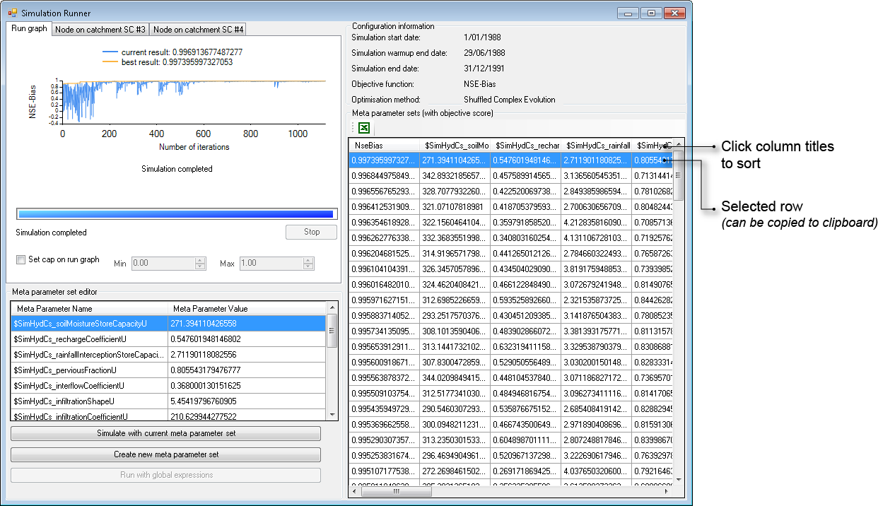
Once a simulation run has been completed, the metaparameter values from the best run are listed in the Meta parameter set editor table (below the graph). You can simulate the model with this parameter set by clicking Simulate with current meta parameter set or choose a different set (click Create new meta parameter set to enter metaparameter values for manual optimisation).
The Meta parameter sets table shows how calibration was configured, and checks the degree of consistency in the calibration runs. The rows of the results table are sorted by objective function. You can click column titles to change the sort order. For example, clicking the left-most column title once sorts the table into ascending order of objective function measure. That is, the first row of the table will reflect the "worst" iteration. Clicking the same column title a second time will sort the table into descending order of objective function measure, so the first row will then contain the "best" iteration.
You can also export the results to Microsoft Excel. Additionally, you can select one row at a time and press Ctrl+C to copy to the clipboard. Note that you cannot select individual cells. You can select also metaparameters values and copy to the clipboard.
To check how well the calibration performed, check the simulation results for other nodes or links by clicking on their respective tabs on the top left of the Simulation Runner dialog (left side of Figure 8). Click on the desired tab, then choose the node from the drop-down menu, and click View. This shows the model and gauge flow in Results Manager. To undertake further investigations for selected periods using logarithmic curves or the Statistics tab, for example, refer to Results Manager.
In addition to calibrating individual values, you can also calibrate a function using the /wiki/spaces/SD50/pages/50136870.