Note: This is documentation for version 5.0 of Source. For a different version of Source, select the relevant space by using the Spaces menu in the toolbar above
Fundamental Concepts
Introduction
Using Source is a two stage process. First models must be built, and then they can be used, or run. Generally, these models can be classified into four categories, although there can be overlaps:
- River system models - these allow users to assess long-term impacts of water resource policy on system storages, flows and water shares, and develop better ways of managing river systems;
- River operations models - assist water authorities to optimise their day-to-day operations, such as water releases to meet irrigation demands and environmental requirements;
- Catchment models - provide information on the source, transport, transformation and fate of nutrients and pollutants. They are commonly used to develop, test and refine management strategies to improve water quality in rivers and reduce loads to receiving waters; and
- Urban models - allow the optimisation of urban supply systems and the development and refinement of water conservation strategies.
There are features common to all models which are described in Representing Systems in Source.
Model workflow
Source modelling comprises of the following four steps:
- Build;
- Calibrate;
- Run; and
- Report.
Building a Source model
Building a model in Source is an iterative process. Once you start building it, you can collect more information, and refine the process and outputs, until ultimately the model is considered ‘fit for purpose’. Generally, a simple model is developed first, and this will continue to be refined for years as new questions or issues arise. The model you are developing now may be still be in use 20 years later, so it is important to be organised, systematic and to document all major decisions. Refer to Guidelines for Water Management Modelling.
The general approach to model building is as follows:
- Draw a schematic diagram representing the basic physical structure to be modelled, refer to adding nodes and adding links to a model. Include the major waterways, stream gauges, inflows, diversions and outflows. You can begin the process of dividing a catchment into sub-catchments;
- Collect data on land use, flows, and other features that are important for your model. For a river system model you will need information on diversions and return flows. For a catchment model, you will need information on nutrient generation rates from different land uses. Urban models will have their own specific data requirements;
- Go back and refine the model schematic to take account of any new data that you have collected;
- Build the model in Source. This is referred to as populating the model because all parameters must be entered and their behaviour specified; and
- Calibrate the operational parameters. The purpose of calibration is to ensure the model is a reasonable representation of the current situation. It is important to be confident about this before testing the effect of any changes. Calibration will need to be revisited if the intended use of the model changes. To calibrate catchment models, refer to Calibration Wizard for catchments.
Simulation phases
Source steps through a series of phases during a scenario run to calculate and record various elements. Named simulation phases, they are executed for every time-step and is detailed here.
Time-steps
The following sections provide an overview of some important features in Source.
About time-steps and time-stamps
For clarity, the following definitions apply:
- Time-stamp - a date and an optional time on that date. A time-stamp represents a moment in time.
- Measurement - a value, for example, a flow measurement would typically have units for megalitres per day.
- Observation - a time-stamp plus at least one associated measurement.
- Time series - a file or database containing a set of observations in monotonically ascending order of time-stamp.
- Time-step - the resolution of the executing model. A time-step is a multiple of whole seconds and represents a duration of time, as distinct from a time-stamp which represents a moment in time.
Source uses the time-stamps in your time-series files to determine the time-step for the model. For example, if your time-series files contain daily time-stamps then Source operates on a daily time-step. For this reason, you need to ensure that all time-series files in a model use the same time-stamp granularity.
The number of seconds, or duration, of a time-step is calculated by subtracting the first second of the current time-step from the first second of the following time-step. When the model is operating in seconds, minutes, days, hours or weeks, the number of seconds in a time-step will always be fixed. For example, a day always contains 86,400 seconds (leap seconds are ignored). However, once time-step granularity reaches a month or more, the number of seconds in a time-step is variable. For example, the number of seconds in a month depends on whether the month contains 31 days; and for February and a whole year, whether the year is a leap year.
When reading a time series, Source assumes that the measurements in each observation were made at the first instant of the associated time-step, and that each measurement stands for the whole of the time-step. The measurements associated with time-stamps are expressed in units that you specify, either in the time series itself or in the feature editor when you load the time series. For example, a common unit would be megalitres per day. Regardless of the units of the original measurement, for internal use, Source converts each value to cubic metres per second using the number of seconds in the time-step.
Source does not interpolate between adjacent observations or otherwise attempt to calculate mean data or moving averages. The single value at the start of the time-step stands for the whole of the time-step.
Figure 6. Time-stamps vs time-steps

The relationships are summarised in Figure 6. Here, the time series of flows contains observations with daily time-stamps so Source adopts a daily time-step. The duration of each time-step is calculated as follows:
Equation 1 | 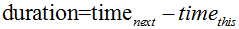 |
|---|
where all values are in seconds. An observation of 40 ML/day time-stamped 22/01/2009 is converted to 0.46 m3/s and that value stands for the whole of the time-step. Note that flows are always converted to m3/s for internal calculations but you can specify the units that are displayed.
It is up to you to ensure that your time-series files respect these assumptions.
Plugins and component models
Source’s capabilities can be extended through the use of plugins, which are data processing tools external to Source.They can be new component models (eg. new rainfall runoff or Water user demand model) and data processing tools that are external to Source.
They can either extend its user interface, or add steps or models to the Geographic Wizard.
Source supports a range of component models. These are mathematical models or algorithms that represent particular physical processes, such as rainfall runoff generation, flow routing or constituent filtering:
- Built-in component models. When you install Source, several component models are installed at the same time and some of these will automatically appear in the menus; others must be loaded manually;
- Component models, such as the River Harvesting Diversion Node model, that can be manually loaded into Source. A range of component models are available where specific user interfaces have been constructed; or
- Plugins are loaded into Source and run alongside a model. You can use these to process data from the output of a Source scenario. These component models are external to Source and must be compatible with the software .
All plugin models and tools listed in this guide have undergone quality assurance and testing procedures endorsed and supported by eWater Ltd. Any issues or problems that may occur with these plugins will be resolved by the Source software development team supported by eWater.
Third party plugins that are compatible with Source are available to download from http://www.toolkit.net.au. These plugins are externally developed through groups and organisations outside of the eWater Source Project and are not supported by eWater or the Source software development team. Using externally developed plugins for purposes outside of their intended use is not recommended or endorsed by eWater.
Instructions on writing a plugin for Source are available from /wiki/spaces/SC/pages/51643422.
Mass balance
Mass balance, or water balance, is based on the principle that water mass is preserved in the river system. It ensures that losses do not exceed inflows and determines whether a model has been calibrated properly. Source ensures that water balance is respected in flow calculations, and mass balance is also respected for calculations involving constituents. Additionally, it has a mass balance reporting functionality, which is a feature that some other models do not have.
Units
This section provides an overview of the units used in Source.
Internal measurement units
River system modelling typically focuses on the distribution, use and mass balance of water volumes within those systems. Accordingly, units for input data (eg time-series files) and results are commonly expressed in volumes per unit time-step for the model (eg. ML/day or GL/month).
In Source, regardless of the original units of the input flow data, the internal computational process is undertaken in cubic metres per second. All input data undergoes unit conversion using the number of seconds in the time-step. Source produces results (accessed via the Recording Manager) and data (for export) expressed in both user-specified units and in m3/s. The results are provided for completeness, so you are given the full picture of what the model:
- does with input data;
- uses to do internal calculations; and
- does to produce output data.
Units drop-down menu
Source provides several options for various units of measurements. A full list can be viewed using , as described in User Preferences and Settings.
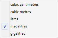
Figure 7 shows an example of volume data units (megalitres as the chosen unit) that are available in Source.
Figure 7. Example units drop-down menu