Note: This is documentation for version 5.4 of Source. For a different version of Source, select the relevant space by using the Spaces menu in the toolbar above
Exponential Decay SRG
Introduction
The Exponential Decay model applies an exponential decay to the stored constituent mass in a node or link.
Scale
This model operates at a river reach scale.
Principal Developer
eWater
Authors
Rachel Blakers, Andrew Davidson
Version
Source v4.1
Availability/Conditions
The Exponential Decay model is automatically installed with Source. For Lumped constituent routing, it can be applied to constituents in:
- Storage Nodes
- Weir Nodes
- Storage Routing Links
For Marker constituent routing, it can be applied to constituents in:
- Storage Nodes
- Weir Nodes
The decay model is not currently available for Storage Routing Links if Marker routing is used.
Definition of Symbols
Symbol | Description |
M(t) | Constituent mass in storage (instantaneous) |
V(t) | Storage volume (instantaneous) |
Qin(t) | Water volume flowing into the storage (instantaneous) |
Cin(t) | Constituent concentration flowing into the storage (instantaneous) |
Qout(t) | Water volume flowing out of the storage (instantaneous) |
Cout(t) | Constituent concentration flowing out of the storage (instantaneous) |
k | Exponential decay constant |
t | Time |
h | Exponential decay half-life (input by user) |
Background
Exponential Decay
Exponential decay describes the decay of a quantity at a rate that is directly proportional to the amount present (Equation 1).
Equation 1 |
|
where M is the quantity and k is the decay constant. Integrating Equation 1 gives a solution for M:
Equation 2 |
|
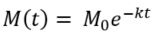
where M0 is the initial quantity.
The decay constant can be expressed in terms of the time taken for the quantity to fall to one half of its initial value. This time is called the half-life, denoted h. It can be shown that the half-life and the decay constant have the following relationship:
Equation 3 |
|
where ln is the natural logarithm.
Substituting Equation 3 into Equation 2 and simplifying gives the following expression for constituent mass:
Equation 4 |
|
Constituent Decay in a Fully Mixed Store
In Source, the model describing the exponential decay of a constituent must consider inflows and outflows from the storage (here the term "storage" is used in a general sense and refers to the water stored in a river reach or reservoir, for example). Assuming instantaneous, fully mixed conditions, the change in constituent mass over time can be determined from the following conservation of mass relationship:
Equation 5 |
|
where k is the decay constant, Qin and Cin are the inflow water volume and constituent concentration, respectively, and Qout and Cout are the outflow water volume and constituent concentration, respectively. Assuming constituent outflows are at the same concentration as the storage (i.e. fully-mixed conditions), we can write Equation 5 as:
Equation 6 |
|
where V is the instantaneous volume of the storage.
Unlike Equation 1, a general solution does not exist for Equation 6. An approximate solution can be derived using the backward (implicit) Euler method, giving:
Equation 7 |
|
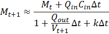
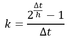
where Mt is the constituent mass at the end of time step t, Vt is the storage volume at the end of time step t, and ![]() is the time step size. Equation 7 assumes that flux rates are constant during a time step and that the storage volume at the end of the time step is representative of the volume during the time step. It is more convenient to express the change in constituent mass with respect to the half-life h. An expression for the half-life can be derived for Equation 7 as:
is the time step size. Equation 7 assumes that flux rates are constant during a time step and that the storage volume at the end of the time step is representative of the volume during the time step. It is more convenient to express the change in constituent mass with respect to the half-life h. An expression for the half-life can be derived for Equation 7 as:
Equation 8 |
|
Using the above expression, we can then express Equation 7 in terms of the half-life rather than the decay constant:
Equation 9 |
|
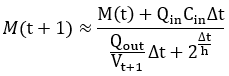
Equation 9 forms the basis of the Exponential Decay model in Source. The solution becomes less accurate as the half-life becomes smaller (particularly if the half-life is smaller than the time step) and as the flushing rate (Qout /Vt+1) becomes larger. It also follows from Equation 9 that if Vt+1 = 0 then Mt+1 = 0.
Trend Concentration and Percent Reduction%
This function allows to decay concentration and then remove the certain percentage of the constituent. The basic formula is the equation 9.
Trend Concentration
It considers two conditions:
(i): Trend Concentration < Concentration at the begging of time step:
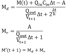
Where:
M'(t+1) is the constituent mass after the process of Trend Concentration
A= V* TrendConcentration is the total mass for the task concentration.
(ii): Trend Concentration > Concentration at the begging of time step
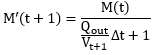
Percent Reduction%
The function will remove the input percent value directly from the processed constituent mass.
Where:
C’(t+1) is the constituent concentration at the storage after the process of Trend Concentration
M’’(t+1) is the sum of the constituent mass after the process of Trend Concentration and in the outflow
M(t+1) is the final constituent mass after the process of Trend Concentration and Percent Reduction.
Example
If the half-life is equal to the time step, then the constituent mass after one time step will be equal to one half of the previous mass (ignoring losses and gains from outflows and inflows). For example, consider a half-life of h = 1 day, a daily time step, zero inflows and zero outflows. Equation 9 tells us that, after 1 day, the constituent mass will be:
![]()
which is one half of the initial mass.
Solution Methodology - Flow Phase
The Exponential Decay model can be applied in Storage and Reservoir nodes for both Marker and Lumped constituent routing. Currently, it can only be applied in Storage Routing Links if Lumped constituent routing is used. The model is run each time step after the flow phase calculations for the relevant node or link:
- For Storage and Weir Nodes, the Exponential Decay model is solved once per time step for the entire storage.
- Storage Routing Links can have one or more divisions, which remember state. Each time step, the Exponential Decay model is solved separately for each division, starting with the division at the head of the link and moving downstream.
The Exponential Decay model is based on Equation 9. However, this equation is derived under the assumption that constituent outflows from the storage are at the same concentration as the storage. In Source, this assumption does not always hold. Evaporation, for example, can completely deplete a storage without removing any constituents. The evaporated volume is subtracted from the storage volume before the Exponential Decay model is applied. As a result, it is possible for the storage volume to be 0 and the constituent mass to be greater than 0, which can give rise to mass balance issues and infinite constituent concentrations. The model addresses zero end-of-time-step storage volumes using a concept of deposited mass L, which is a constituent mass deposited on the riverbed and lost to the system. The solution procedure is as follows:
CASE 1: If the end-of-time-step storage volume is 0 and the outflow is 0, then all constituent mass is deposited.
CASE 2: If the end-of-time-step storage volume is 0 and the outflow is greater than 0, then all constituent mass leaves the storage with the outflow.
CASE 3: If the end-of-time-step storage volume is greater than 0, then Equation 9 applies.
|
Input Data
A single value for the half-life parameter in seconds. Smith et al. (2011) provide some estimates of pesticide half-lives, Birgand et al. (2007) and Rao et al. (2009) provide estimates of decay rates for nutrients in streams.
Parameters or Settings
Model parameters are summarised in Table 1.
Table 1. Decay model parameters.
Parameter | Description | Units | Default | Range |
Half-life | The half-life of the constituent | seconds | 86400 (equivalent to 1 day) | 0 to ∞ |
| Percent Reduction | A percent value that the user wishes to remove directly from the processed constituent | % | 0 | 0 to 100 |
| Trend Concentration | The concentration to trend down to | mg/L | 0 | 0 to ∞ |
Outputs
A time series of stored constituent mass.
Reference List
Birgand, F., R.W. Skaggs, G.M. Chescheir, J.W. Gilliam (2007) Nitrogen Removal in Streams of Agricultural Catchments-A Literature Review. Critical Reviews in Environmental Science and Technology; 2007; 37, 5; ProQuest Agriculture Journals, p. 381
Rao, P.S.C., N.B. Basu, S. Zanardo, G. Botter, A. Rinaldo (2009) Contaminant load-discharge relationships across scales in engineered catchments: Order out of complexity. 18th World IMACS / MODSIM Congress, Cairns, Australia 13-17 July 2009, p. 1886-1892. http://mssanz.org.au/modsim09
Smith, R., R. Turner, S. Vardy, M. Warne (2011) Using a convolution integral model for assessing pesticide dissipation time at the end of catchments in the Great Barrier Reef Australia. In F. Chan, D. Marinova, R.S. Anderssen (eds) Modsim2011, 19th International Congress on Modelling and Simulation. Modelling and Simulation Society of Australia and New Zealand, December 2011, pp. 2064-2070. ISBN: 978-0-9872143-1-7. http://www.mssanz.org.au/modsim2011/E5/smith.pdf